Script 04 — MEGPath Production Results

Parse, visualize, and interpret NMF factors from MEGPath runs

Background

Scripts 01–03 screened preprocessing approaches using R’s NMF package. The best candidates were then run through MEGPath — the production C++ NMF algorithm (Dyer & Dymacek 2018) that uses Monte Carlo Markov Chain + simulated annealing. MEGPath normalizes each input matrix to [0, 1] internally and minimizes LAD (Least Absolute Deviation = $\sum|V - WH|$).

We compiled MEGPath locally and ran 8 configurations at 100K iterations each:

Configuration	Matrix	k	Rows
scRNA Baseline	Ethan’s `dense_dataLT.csv` (double-log, all 17,857 genes)	2, 3	17,857
scRNA Improved	SCTransform + 2,000 HVGs	2, 3	2,000
TCR Baseline	Ethan’s `tcr_expansion.csv` (all 2,541 clonotypes)	2, 3	2,541
TCR Improved	Bio Filter C (Expanded $\cup$ TIL-observed, 416 clonotypes)	2, 3	416

Reproducing these runs

MEGPath is installed permanently at megpath/ within this project (with Eigen 3.4.0 bundled at megpath/eigen-3.4.0/). To rerun or add new configurations:

# MinGW must be in PATH for runtime libraries
export PATH="/c/Users/mattj/AppData/Local/Microsoft/WinGet/Packages/BrechtSanders.WinLibs.POSIX.UCRT_Microsoft.Winget.Source_8wekyb3d8bbwe/mingw64/bin:$PATH"

# Run from megpath_runs/ directory
cd megpath_runs
../megpath/standard/connmf.exe -a args_tcr_baseline_k2.txt

Argument files specify the input CSV, rank (via one_patterns — number of empty strings = k), output directory, and iteration count. Pre-create the output directory before running (mkdir -p ./output_dir/). Set stats = "all" or no output files are written. File paths must not contain spaces (MEGPath crashes on them).

To recompile after modifying source:

cd megpath/shared && mingw32-make clean && mingw32-make
cd ../standard && mingw32-make clean && mingw32-make

This script parses the MEGPath output files, extracts the H matrix (temporal patterns: how each factor behaves across the 4 timepoints) and W matrix (gene/clonotype loadings: which features belong to each factor), and interprets the results biologically.

Code

library(ggplot2)
library(dplyr)
library(reshape2)
library(readr)
source("theme_donq.R")

timepoints <- c("Pre", "Wk3", "Wk6", "Wk9")

1. Parse MEGPath Output Files

MEGPath output format:

Header lines (#): metadata + H matrix (patterns $\times$ timepoints), space-separated
Data lines: row-id, W[0], W[1], ..., W[k-1], row_error — W matrix coefficients followed by the per-row reconstruction error

Code

parse_megpath <- function(filepath) {
  lines <- readLines(filepath)

  # --- Metadata ---
  meta <- list()
  meta$file <- gsub("^#File : ", "", lines[grep("^#File", lines)])
  meta$n_genes <- as.integer(gsub("^#Number_of_genes : ", "", lines[grep("^#Number_of_genes", lines)]))
  meta$max_runs <- as.integer(gsub("^#MAX_RUNS : ", "", lines[grep("^#MAX_RUNS", lines)]))
  meta$k <- as.integer(gsub("^#Num_Patterns : ", "", lines[grep("^#Num_Patterns", lines)]))
  meta$total_error <- as.numeric(gsub("^#Total_error : ", "", lines[grep("^#Total_error", lines)]))
  meta$runtime <- gsub("^#Total_running_time : ", "", lines[grep("^#Total_running_time", lines)])

  # --- H matrix (patterns) ---
  # Lines like: #"",0.464416 0.464727  0.46484 0.464863
  h_lines <- grep('^#"",', lines, value = TRUE)
  H <- do.call(rbind, lapply(h_lines, function(l) {
    vals <- gsub('^#"",', '', l)
    as.numeric(strsplit(trimws(vals), "\\s+")[[1]])
  }))
  colnames(H) <- c("Pre", "Wk3", "Wk6", "Wk9")
  rownames(H) <- paste0("Factor_", 1:nrow(H))

  # --- W matrix (coefficients) + per-row error ---
  data_lines <- grep("^row-", lines, value = TRUE)
  parsed <- do.call(rbind, lapply(data_lines, function(l) {
    parts <- strsplit(l, ",")[[1]]
    as.numeric(parts[-1])  # drop row-id
  }))

  k <- meta$k
  W <- parsed[, 1:k, drop = FALSE]
  row_errors <- parsed[, k + 1]

  colnames(W) <- paste0("Factor_", 1:k)

  list(meta = meta, H = H, W = W, row_errors = row_errors)
}

Code

runs <- list(
  scrna_baseline_k2 = "megpath_runs/scrna_baseline_k2/one_results.csv",
  scrna_baseline_k3 = "megpath_runs/scrna_baseline_k3/one_results.csv",
  scrna_sct2k_k2    = "megpath_runs/scrna_sct2k_k2/one_results.csv",
  scrna_sct2k_k3    = "megpath_runs/scrna_sct2k_k3/one_results.csv",
  tcr_baseline_k2   = "megpath_runs/tcr_baseline_k2/one_results.csv",
  tcr_baseline_k3   = "megpath_runs/tcr_baseline_k3/one_results.csv",
  tcr_bio_k2        = "megpath_runs/tcr_bio_k2/one_results.csv",
  tcr_bio_k3        = "megpath_runs/tcr_bio_k3_full/one_results.csv"
)

results <- lapply(runs, parse_megpath)

2. Error Comparison

Code

summary_df <- do.call(rbind, lapply(names(results), function(name) {
  m <- results[[name]]$meta
  data.frame(
    Run = name,
    Data = ifelse(grepl("scrna", name), "scRNA", "TCR"),
    Matrix = ifelse(grepl("baseline", name), "Baseline", "Improved"),
    k = m$k,
    Rows = m$n_genes,
    LAD = round(m$total_error, 1),
    LAD_per_element = round(m$total_error / (m$n_genes * 4), 5),
    Runtime = m$runtime,
    stringsAsFactors = FALSE
  )
}))

knitr::kable(summary_df, caption = "MEGPath Production Results (100K iterations)")

MEGPath Production Results (100K iterations)
Run	Data	Matrix	k	Rows	LAD	LAD_per_element	Runtime
scrna_baseline_k2	scRNA	Baseline	2	17857	452.0	0.00633	0d0h26m35.285s
scrna_baseline_k3	scRNA	Baseline	3	17857	237.3	0.00332	0d0h42m28.254s
scrna_sct2k_k2	scRNA	Improved	2	2000	14.1	0.00176	0d0h2m51.015s
scrna_sct2k_k3	scRNA	Improved	3	2000	14.1	0.00177	0d0h4m25.178s
tcr_baseline_k2	TCR	Baseline	2	2541	20.5	0.00202	0d0h3m38.207s
tcr_baseline_k3	TCR	Baseline	3	2541	20.2	0.00199	0d0h5m44.855s
tcr_bio_k2	TCR	Improved	2	416	5.4	0.00327	0d0h0m35.94s
tcr_bio_k3	TCR	Improved	3	416	5.2	0.00315	0d0h0m55.798s

Code

plot_df <- summary_df %>%
  mutate(Label = paste0(Matrix, " k=", k),
         Label = factor(Label, levels = unique(Label)))

ggplot(plot_df, aes(x = Label, y = LAD_per_element, fill = Matrix)) +
  geom_col(width = 0.6) +
  geom_text(aes(label = sprintf("%.5f", LAD_per_element)),
            vjust = -0.5, color = "#b0b0b0", size = 3.5) +
  facet_wrap(~Data, scales = "free") +
  scale_fill_manual(values = c("Baseline" = "#555555", "Improved" = "#ffffff")) +
  labs(title = "MEGPath Error per Element: Baseline vs Improved",
       subtitle = "Lower = better reconstruction. 100K simulated annealing iterations.",
       x = NULL, y = "LAD / (rows × columns)") +
  theme_donq() +
  theme(legend.position = "none",
        axis.text.x = element_text(angle = 30, hjust = 1))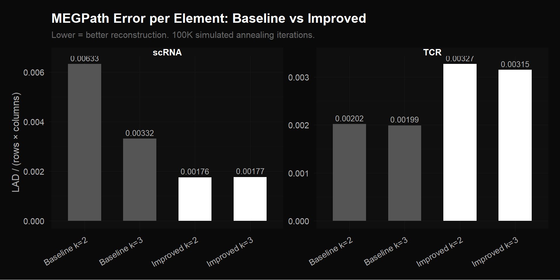

scRNA (left panel): Our preprocessing — SCTransform normalization + filtering to 2,000 highly variable genes — cuts error per element by 47% compared to Ethan’s baseline (0.00177 vs 0.00332). The improved k=2 and k=3 bars are identical, meaning 2 factors fully describe the improved matrix and a 3rd adds nothing. The baseline k=2 is worst (0.00633) because 2 factors can’t fit the noise structure in 17,857 genes; baseline k=3 is better but still ~2x worse than improved. The improved matrix also runs 10x faster (3 min vs 42 min).

TCR (right panel): The bio-filtered bars are taller than baseline — this is not a failure. Most of the 2,541 baseline clonotypes are present at a single timepoint (96% zeros), so they’re trivially easy to reconstruct (just predict zero). Removing them leaves 416 clonotypes with actual temporal dynamics, which are harder to compress but carry the real biological signal.

Code

# scRNA: labeled CSV has gene names as row names
scrna_labels <- read.csv("megpath_inputs/scrna_sct_hvg2k_labeled.csv",
                         row.names = 1, check.names = FALSE)
gene_names <- rownames(scrna_labels)

# TCR bio: read from Table S8 and apply Filter C
# S8 uses "Expanded" / "TIL.observed" as column values (not "Yes")
library(readxl)

Warning: package 'readxl' was built under R version 4.5.2

Code

s8 <- read_excel("NMF Research Data/crc-22-0383-s01.xlsx",
                 sheet = "Table S8", skip = 4)
is_expanded <- !is.na(s8[["Expanded"]]) & s8[["Expanded"]] == "Expanded"
is_til <- !is.na(s8[["TIL.observed"]]) & s8[["TIL.observed"]] == "TIL.observed"
bio_idx <- which(is_expanded | is_til)
bio_clones <- s8[["TCRB.clonotype"]][bio_idx]

3. scRNA: Flat Temporal Patterns Reveal a Pseudobulk Limitation

3a. H Matrix — No Temporal Signal

The H matrix shows how each NMF factor’s weight varies across the 4 timepoints. If NMF discovers temporal programs (e.g., “genes that rise during treatment”), the H matrix lines should diverge across timepoints.

Code

H_k2 <- results$scrna_sct2k_k2$H
h_df <- melt(H_k2)
colnames(h_df) <- c("Factor", "Timepoint", "Weight")
h_df$Timepoint <- factor(h_df$Timepoint, levels = timepoints)

ggplot(h_df, aes(x = Timepoint, y = Weight, group = Factor, color = Factor)) +
  geom_line(linewidth = 1.2) +
  geom_point(size = 3) +
  scale_color_donq() +
  labs(title = "scRNA Temporal Patterns (k=2)",
       subtitle = "H matrix from SCT+2k HVGs — how each factor varies over treatment",
       y = "Pattern weight") +
  theme_donq()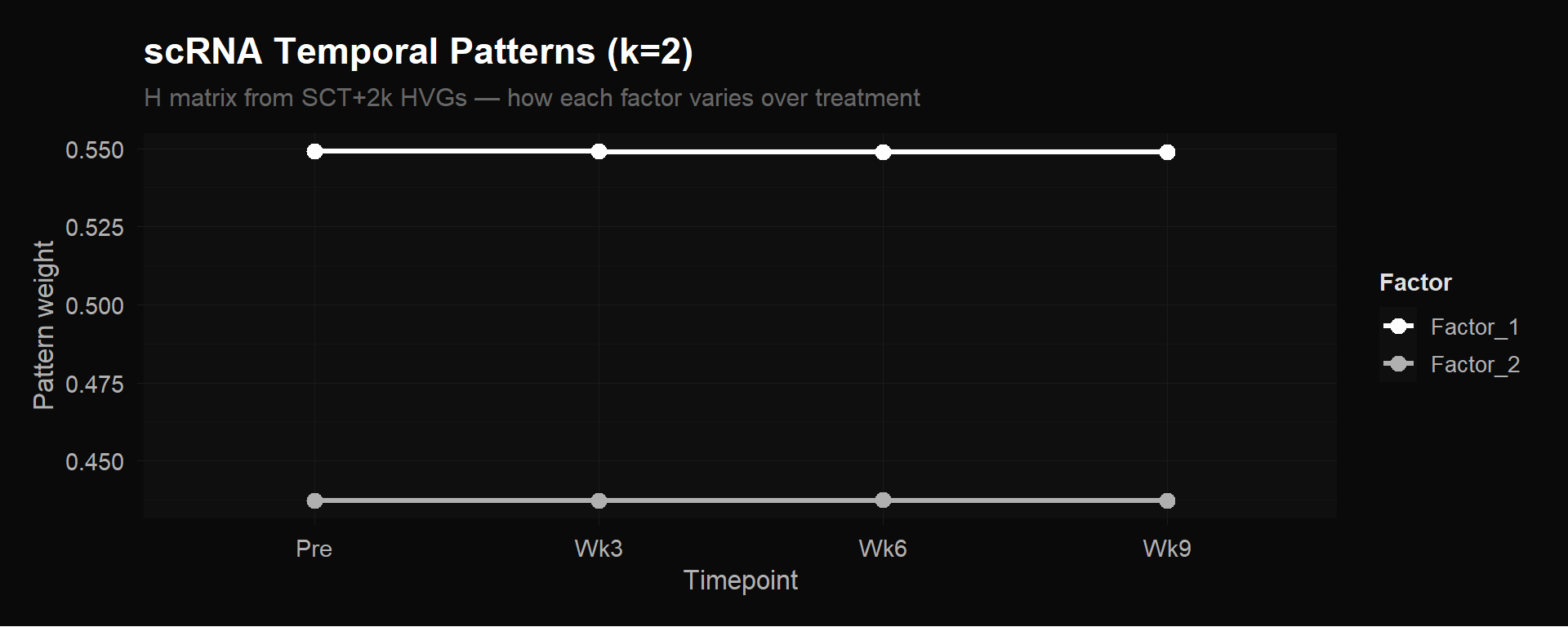

Code

H_k3 <- results$scrna_sct2k_k3$H
h_df3 <- melt(H_k3)
colnames(h_df3) <- c("Factor", "Timepoint", "Weight")
h_df3$Timepoint <- factor(h_df3$Timepoint, levels = timepoints)

ggplot(h_df3, aes(x = Timepoint, y = Weight, group = Factor, color = Factor)) +
  geom_line(linewidth = 1.2) +
  geom_point(size = 3) +
  scale_color_donq() +
  labs(title = "scRNA Temporal Patterns (k=3)",
       subtitle = "H matrix from SCT+2k HVGs — identical total error to k=2",
       y = "Pattern weight") +
  theme_donq()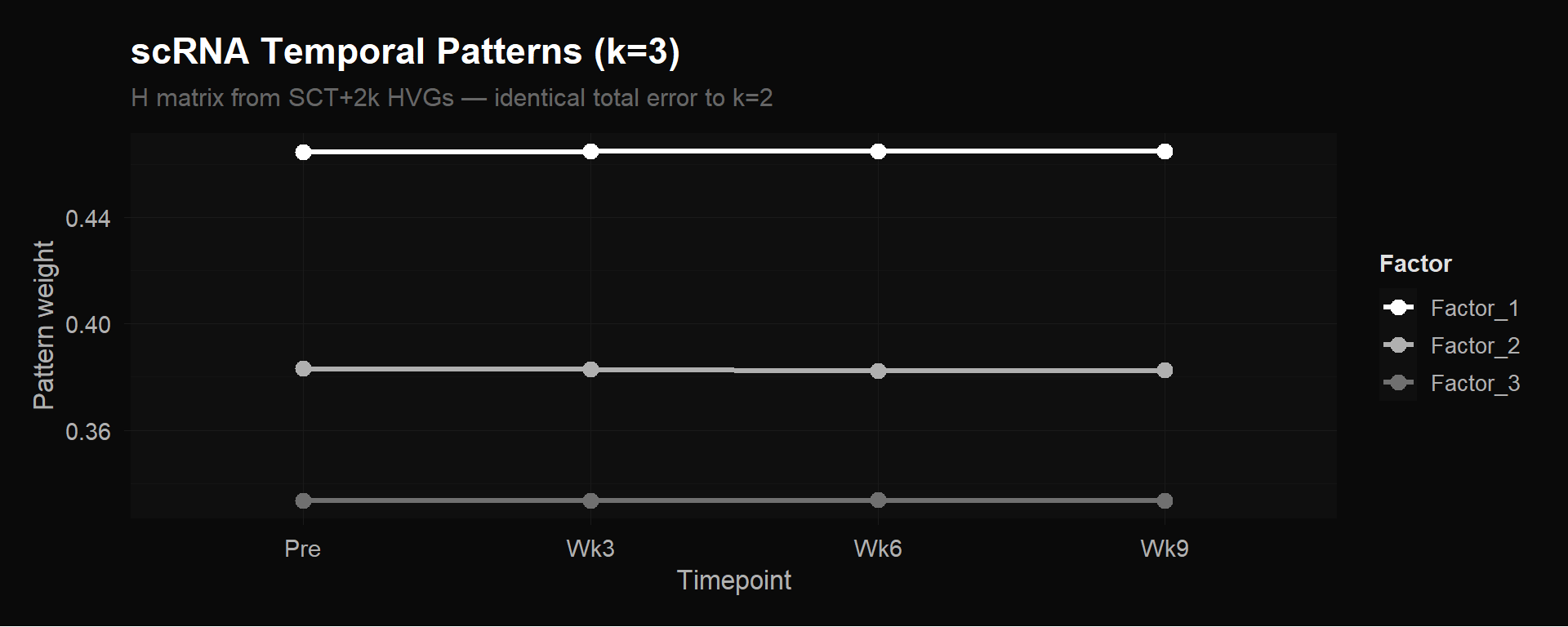

Both plots show perfectly flat lines. Factor 1 sits at ~0.549 and Factor 2 at ~0.437 across all four timepoints (k=2). Adding a third factor (k=3) just splits the weights into three flat lines (~0.465, ~0.383, ~0.333) without reducing error.

NMF found zero temporal variation in the pseudobulk scRNA matrix. This doesn’t mean gene expression doesn’t change during treatment — it means that averaging all ~4,876 cells per timepoint into a single column buries the signal. The CX3CR1+ effectors that expand are a few hundred cells out of thousands. Their increase gets diluted by the much larger number of cells (naive, memory, etc.) that don’t change. The pseudobulk average barely moves, so the H matrix stays flat.

Implication: Pseudobulk scRNA with only 4 columns is insufficient for temporal NMF. To recover cell-type-specific temporal signals, we would need a genes $\times$ (timepoint $\times$ cluster) matrix (e.g., 2,000 $\times$ 52) that preserves within-timepoint heterogeneity.

3b. W Matrix — NMF Separates Expression Programs, Not Temporal Ones

Since the H matrix is flat, NMF isn’t separating “genes that change over time.” Instead, it’s decomposing the expression matrix into two static expression programs — grouping genes by their overall abundance pattern.

Code

# Use k=2 since it's the more parsimonious model (same error as k=3)
W_scrna <- results$scrna_sct2k_k2$W

# Assign gene names
rownames(W_scrna) <- gene_names

# For each factor, find top 20 genes by loading
for (f in 1:ncol(W_scrna)) {
  top <- sort(W_scrna[, f], decreasing = TRUE)[1:20]
  cat(sprintf("\n=== Factor %d: Top 20 Genes ===\n", f))
  cat(paste(sprintf("  %s: %.4f", names(top), top), collapse = "\n"), "\n")
}


=== Factor 1: Top 20 Genes ===
  RASSF6: 0.8836
  AL590807.1: 0.8816
  EEF1A1: 0.8784
  PDE3B: 0.8598
  PRSS23: 0.8485
  CPT1C: 0.8448
  AC009093.2: 0.8370
  AC051619.8: 0.8361
  ITGA4: 0.8346
  NEXN: 0.8320
  AL591623.1: 0.8304
  AC027031.2: 0.8298
  GADD45B: 0.8268
  MT-ND5: 0.8235
  TIGIT: 0.8228
  KNL1: 0.8183
  IL7R: 0.8175
  AC100835.1: 0.8162
  SH3BGRL3: 0.8096
  CTSW: 0.8090 

=== Factor 2: Top 20 Genes ===
  RPS12: 0.9513
  EEF1A1: 0.9131
  RPL10: 0.8948
  RPS4X: 0.8504
  RPS15A: 0.8429
  RPS3A: 0.8387
  ZNF66: 0.8055
  AL138963.4: 0.7882
  RPLP1: 0.7786
  TPT1: 0.7557
  RTKN2: 0.7549
  PPP1R15A: 0.7497
  RPS28: 0.7474
  RPL30: 0.7471
  RPS23: 0.7426
  MT2A: 0.7330
  H3F3B: 0.7313
  KRTAP16-1: 0.7310
  CBLN3: 0.7271
  AL590133.1: 0.7260

Code

# Get top 15 genes per factor
top_n <- 15
top_genes <- unique(unlist(lapply(1:ncol(W_scrna), function(f) {
  names(sort(W_scrna[, f], decreasing = TRUE))[1:top_n]
})))

W_top <- W_scrna[top_genes, , drop = FALSE]
w_df <- melt(W_top)
colnames(w_df) <- c("Gene", "Factor", "Loading")

# Mark known biology genes
bio_genes <- c("CX3CR1", "GZMB", "GZMH", "PRF1", "NKG7", "CCL4", "CCL5",  # cytotoxicity
               "LAG3", "TIGIT", "PDCD1", "HAVCR2", "CTLA4",                 # exhaustion
               "MKI67", "TOP2A",                                             # proliferation
               "TCF7", "SELL", "CCR7", "LEF1",                               # naive/memory
               "GZMK", "CXCR3",                                              # early effector
               "GNLY", "IFNG")                                               # effector cytokines
w_df$Biology <- ifelse(w_df$Gene %in% bio_genes, "Known marker", "")

ggplot(w_df, aes(x = Factor, y = reorder(Gene, Loading), fill = Loading)) +
  geom_tile(color = "#1a1a1a") +
  geom_text(aes(label = ifelse(Biology != "", "*", "")),
            color = "#ffffff", size = 5, vjust = 0.3) +
  scale_fill_donq_heatmap() +
  labs(title = "scRNA W Matrix: Gene Loadings (k=2)",
       subtitle = "Top 15 genes per factor. * = known biology marker.",
       x = "NMF Factor", y = NULL) +
  theme_donq() +
  theme(axis.text.y = element_text(size = 9))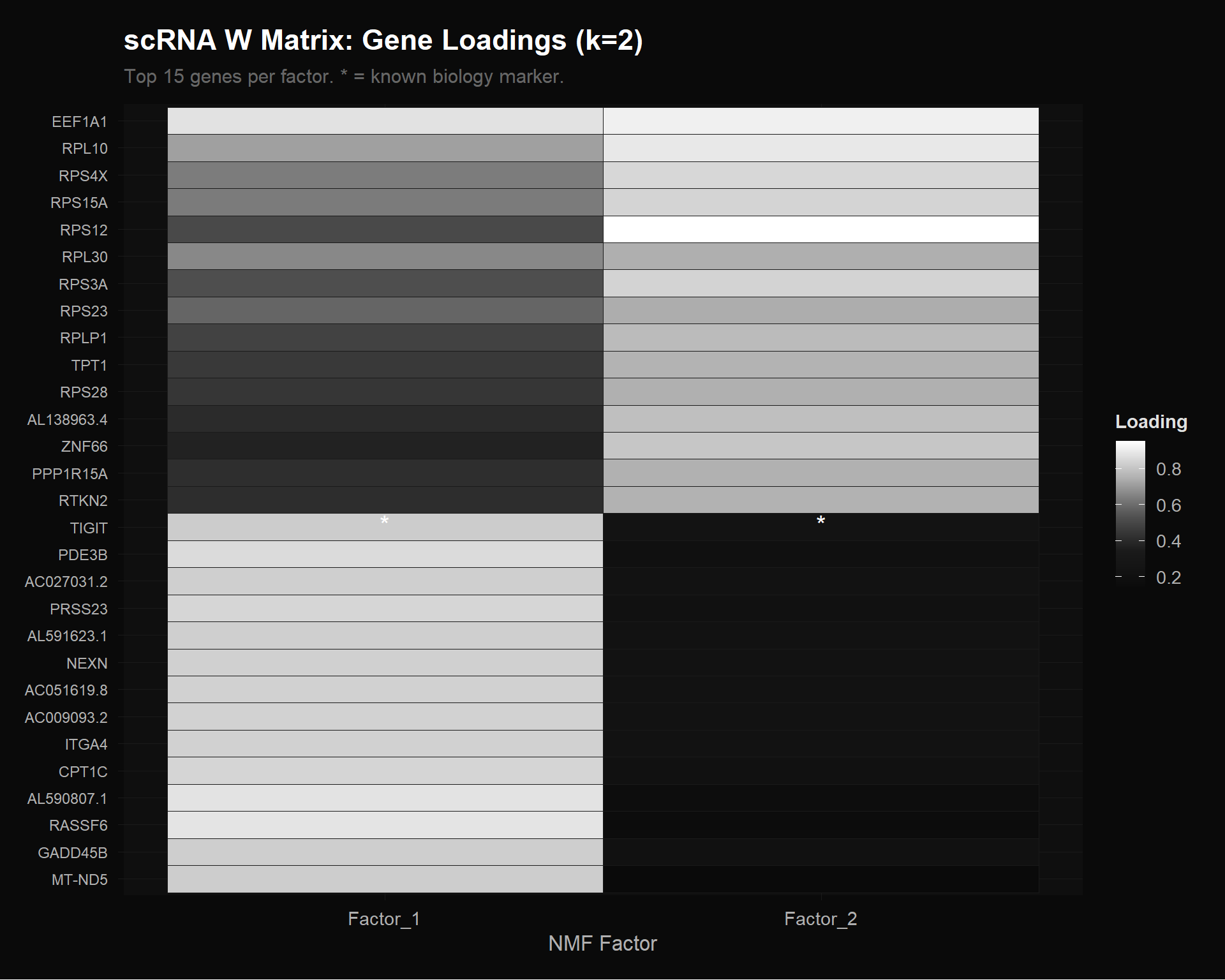

Factor 2 is dominated by ribosomal protein genes: RPS12, RPL10, RPS4X, RPS15A, RPS3A, RPL30, RPLP1, RPS28, RPS23. These are housekeeping translation machinery — the “general cell maintenance” program.

Factor 1 contains more immune-relevant genes: TIGIT (immune checkpoint), IL7R (T cell survival), CTSW (cytotoxic lymphocyte protease), GADD45B (stress response), ITGA4 (integrin). This captures the “immune/functional” program.

3c. Biology Gene Factor Assignments

Code

bio_in_matrix <- intersect(bio_genes, gene_names)
cat("Biology genes found in 2k HVGs:", length(bio_in_matrix), "/", length(bio_genes), "\n\n")

Biology genes found in 2k HVGs: 19 / 22

Code

if (length(bio_in_matrix) > 0) {
  bio_W <- W_scrna[bio_in_matrix, , drop = FALSE]
  bio_assignment <- data.frame(
    Gene = bio_in_matrix,
    Factor_1 = round(bio_W[, 1], 4),
    Factor_2 = round(bio_W[, 2], 4),
    Dominant = apply(bio_W, 1, which.max),
    stringsAsFactors = FALSE
  )
  bio_assignment <- bio_assignment[order(bio_assignment$Dominant, -bio_assignment[, 2 + 1]), ]
  knitr::kable(bio_assignment, caption = "Biology marker genes: factor assignments",
               row.names = FALSE)
}

Biology marker genes: factor assignments
Gene	Factor_1	Factor_2	Dominant
NKG7	0.6376	0.6095	1
GNLY	0.6122	0.5682	1
PRF1	0.5739	0.5642	1
MKI67	0.5662	0.5603	1
SELL	0.6180	0.5101	1
GZMK	0.6132	0.4942	1
CX3CR1	0.6342	0.4807	1
CCR7	0.6325	0.4776	1
LEF1	0.6874	0.4265	1
GZMH	0.7305	0.4033	1
GZMB	0.7085	0.4001	1
TCF7	0.7008	0.3835	1
TIGIT	0.8228	0.2395	1
IFNG	0.4646	0.6913	2
CCL5	0.5704	0.6905	2
CXCR3	0.5188	0.6120	2
CTLA4	0.5275	0.6084	2
CCL4	0.5545	0.6023	2
LAG3	0.5590	0.5715	2

Nearly all biology markers load onto Factor 1, but the margins are slim — e.g., NKG7 loads 0.638 on F1 vs 0.610 on F2 (a ~5% difference). Both cytotoxic markers (GZMB, GZMH, PRF1) and naive/memory markers (TCF7, LEF1, SELL) end up in the same factor. This confirms NMF isn’t finding functional programs here, just a coarse split between “immune genes” (F1) and “housekeeping genes” (F2).

The exceptions are interesting: IFNG, CCL5, CXCR3, and CTLA4 load more on Factor 2 (the ribosomal factor). These are activation/exhaustion markers, suggesting some coupling between T cell activation and translational activity.

4. TCR: Three Distinct Temporal Programs

This is where the biology is. Unlike the flat scRNA patterns, the TCR H matrix shows genuine temporal dynamics — NMF discovered three distinct clonotype expansion behaviors.

4a. H Matrix — Three Temporal Programs (k=3)

Code

H_tcr3 <- results$tcr_bio_k3$H
h_tcr <- melt(H_tcr3)
colnames(h_tcr) <- c("Factor", "Timepoint", "Weight")
h_tcr$Timepoint <- factor(h_tcr$Timepoint, levels = timepoints)

ggplot(h_tcr, aes(x = Timepoint, y = Weight, group = Factor, color = Factor)) +
  geom_line(linewidth = 1.2) +
  geom_point(size = 3) +
  scale_color_donq() +
  labs(title = "TCR Temporal Patterns (Bio Filter C, k=3)",
       subtitle = "H matrix — 416 expanded/TIL-observed clonotypes",
       y = "Pattern weight") +
  theme_donq()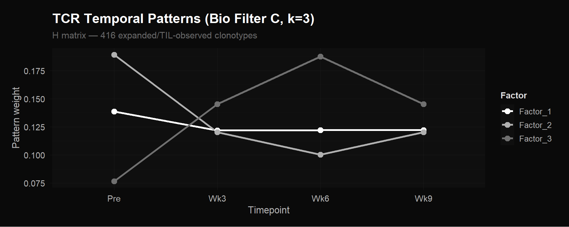

The three factors capture three biologically distinct clonotype behaviors:

Factor 1 (~0.139 at Pre, drops to ~0.122 and stays flat): The “stable/persistent” pattern. Clonotypes that maintain roughly constant frequency throughout treatment. Likely memory or homeostatic clones unaffected by therapy.
Factor 2 (highest at Pre ~0.189, drops sharply to ~0.120 by Wk3, lowest at Wk6 ~0.100, partial recovery at Wk9): The “pre-treatment dominant / contracting” pattern. Clonotypes abundant before treatment that decline during therapy. These are bystander clones being displaced as treatment-responsive clones expand.
Factor 3 (lowest at Pre ~0.077, rises to ~0.145 at Wk3, peaks at ~0.187 at Wk6, then falls to ~0.145 at Wk9): The “treatment-responsive expansion” pattern. Clonotypes that are rare or absent pre-treatment and expand dramatically during chemo-immunotherapy, peaking at week 6.

The week 6 peak in Factor 3 is the key result. Abdelfatah et al. showed that a $$10% increase in CX3CR1+ CD8+ T cells from baseline (“CX3CR1 score”) at 6 weeks predicts treatment response with 85.7% accuracy. NMF independently rediscovered the same timing from clonotype frequency data alone — Factor 3 peaks at exactly the same timepoint, without any prior knowledge of CX3CR1 or response status.

4b. Two-Factor Version (k=2)

Code

H_tcr2 <- results$tcr_bio_k2$H
h_tcr2 <- melt(H_tcr2)
colnames(h_tcr2) <- c("Factor", "Timepoint", "Weight")
h_tcr2$Timepoint <- factor(h_tcr2$Timepoint, levels = timepoints)

ggplot(h_tcr2, aes(x = Timepoint, y = Weight, group = Factor, color = Factor)) +
  geom_line(linewidth = 1.2) +
  geom_point(size = 3) +
  scale_color_donq() +
  labs(title = "TCR Temporal Patterns (Bio Filter C, k=2)",
       subtitle = "H matrix — 416 expanded/TIL-observed clonotypes",
       y = "Pattern weight") +
  theme_donq()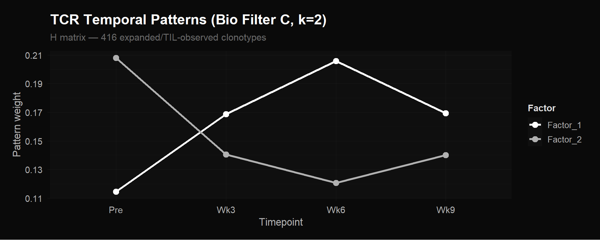

With k=2 the same biology simplifies into a clean X-shaped crossover:

Factor 1 rises from 0.114 $\rightarrow$ 0.169 $\rightarrow$ 0.206 $\rightarrow$ 0.169 = expansion (peaks Wk6)
Factor 2 falls from 0.208 $\rightarrow$ 0.140 $\rightarrow$ 0.121 $\rightarrow$ 0.140 = contraction (trough Wk6)

This captures the fundamental expansion-vs-contraction dichotomy. The k=3 version refines this by splitting Factor 1 into “stable” and “expanding” populations.

4c. W Matrix — Top Clonotypes per Factor

Code

W_tcr <- results$tcr_bio_k3$W

# Verify label count matches W matrix rows
if (length(bio_clones) == nrow(W_tcr)) {
  rownames(W_tcr) <- bio_clones
  tcr_labeled <- TRUE
} else {
  cat("WARNING: Label mismatch! bio_clones:", length(bio_clones),
      "vs W rows:", nrow(W_tcr), "\n")
  rownames(W_tcr) <- paste0("clone_", seq_len(nrow(W_tcr)))
  tcr_labeled <- FALSE
}

for (f in 1:ncol(W_tcr)) {
  top <- sort(W_tcr[, f], decreasing = TRUE)[1:10]
  cat(sprintf("\n=== Factor %d: Top 10 Clonotypes ===\n", f))
  cat(paste(sprintf("  %s: %.4f", names(top), top), collapse = "\n"), "\n")
}


=== Factor 1: Top 10 Clonotypes ===
  CASSSLGSFDEQFF: 0.9983
  CASSQDRGWGLNTEAFF: 0.3612
  CASSEGSATDTQYF: 0.3608
  CASSSHPGQGSNQPQHF: 0.3595
  CASSLPLLAGETQYF: 0.3416
  CASSPILNRGGNEQFF: 0.3359
  CASSQVQGALAGYTF: 0.3322
  CASSEASGTRGSSYGYTF: 0.3310
  CASSLREGYGYTF: 0.3243
  CASSLVGTGDWDTEAFF: 0.3221 

=== Factor 2: Top 10 Clonotypes ===
  CASSSLGSFDEQFF: 0.8967
  CASSLAGTGYEQYF: 0.3614
  CASSVPSGGNEQFF: 0.3599
  CASSSTRFSTGELFF: 0.3598
  CASSLPGGYGYTF: 0.3588
  CASSLGGTGDNEQFF: 0.3573
  CASIPAGRTDTQYF: 0.3549
  CASSLGGGGDTDTQYF: 0.3522
  CASSQDTDRVRSEAFF: 0.3333
  CAWRTGGKVRTEAFF: 0.3297 

=== Factor 3: Top 10 Clonotypes ===
  CASSSLGSFDEQFF: 0.9992
  CASSYRGRSTGELFF: 0.9166
  CASSQVRRGNYGYTF: 0.7162
  CSVEERWTLTEAFF: 0.7017
  CASSYTGFEQYF: 0.6953
  CASSGRYEQYF: 0.6732
  CASSIGTSTDTQYF: 0.6579
  CASSQPEQFF: 0.5137
  CAYYRTGTNPYAQYF: 0.4222
  CASSSSRGISTDTQYF: 0.3651

CASSSLGSFDEQFF (the dominant expander: 13 $\rightarrow$ 20 $\rightarrow$ 81 $\rightarrow$ 28 cells) tops all three factors because it’s so abundant it contributes to every pattern. Factor 3 uniquely captures the key treatment-responsive clonotypes from the paper: CASSYRGRSTGELFF (0.917), CSVEERWTLTEAFF (0.702), CASSYTGFEQYF (0.695), CASSGRYEQYF (0.673).

4d. Clonotype Trajectories by Factor

Code

# Assign each clonotype to its dominant factor
dominant_factor <- apply(W_tcr, 1, which.max)
max_loading <- apply(W_tcr, 1, max)

# How many clonotypes per factor?
factor_counts <- table(dominant_factor)
cat("Clonotypes per factor:\n")

Clonotypes per factor:

Code

print(factor_counts)

dominant_factor
  1   2   3 
158 142 116

Code

# Get the original frequency data to show trajectories
tcr_freq <- read.csv("megpath_inputs/tcr_bio_freq.csv", header = FALSE)
colnames(tcr_freq) <- timepoints
if (tcr_labeled) rownames(tcr_freq) <- bio_clones

# Top 5 clonotypes per factor by loading, plot trajectories
top_per_factor <- lapply(1:3, function(f) {
  idx <- which(dominant_factor == f)
  loadings <- W_tcr[idx, f]
  names(sort(loadings, decreasing = TRUE))[1:min(5, length(idx))]
})

traj_clones <- unlist(top_per_factor)
traj_df <- tcr_freq[traj_clones, ]
traj_df$Clonotype <- rownames(traj_df)
traj_df$Factor <- paste0("Factor_", dominant_factor[traj_clones])
traj_long <- melt(traj_df, id.vars = c("Clonotype", "Factor"),
                  variable.name = "Timepoint", value.name = "Frequency")
traj_long$Timepoint <- factor(traj_long$Timepoint, levels = timepoints)

ggplot(traj_long, aes(x = Timepoint, y = Frequency, group = Clonotype, color = Factor)) +
  geom_line(linewidth = 0.8, alpha = 0.8) +
  geom_point(size = 2) +
  facet_wrap(~Factor, scales = "free_y") +
  scale_color_donq() +
  labs(title = "Top Clonotype Trajectories by NMF Factor",
       subtitle = "Top 5 clonotypes per factor (by W loading). Bio Filter C, k=3.",
       y = "Frequency (% of repertoire)") +
  theme_donq() +
  theme(legend.position = "none")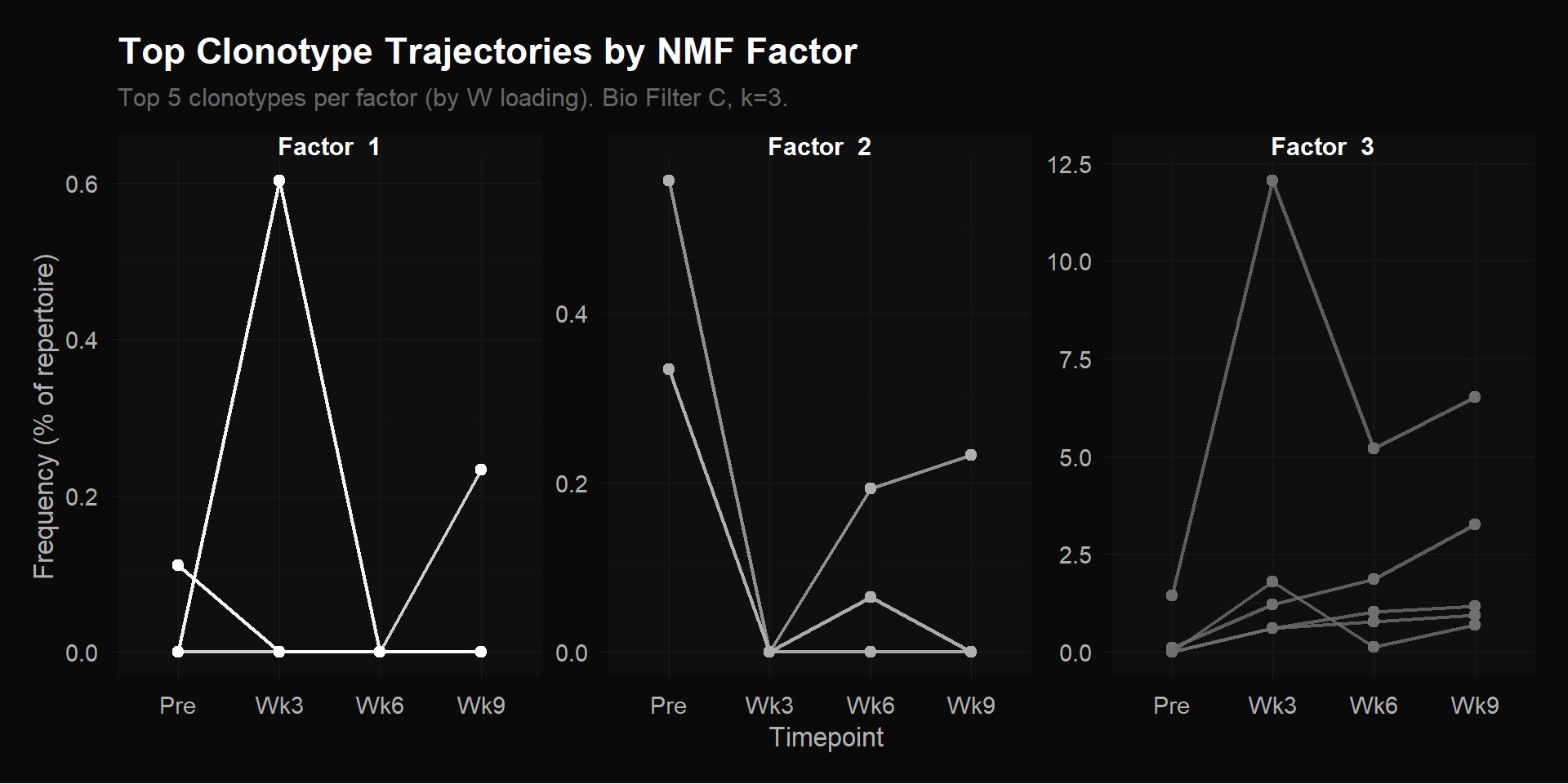

The trajectory plot confirms the H matrix interpretation with the actual clonotype data:

Factor 1 clonotypes: Spike at Wk3 then collapse back to near-zero. These are early transient responders — they expand quickly after treatment initiation but don’t sustain. This may represent an initial immune activation wave that fades.
Factor 2 clonotypes: Start high pre-treatment and drop sharply by Wk3. These are pre-existing clones being displaced as treatment reshapes the TCR repertoire. Classic bystander clonotypes that contract when treatment-responsive clones expand.
Factor 3 clonotypes: Low or absent pre-treatment, dramatic rise peaking at Wk3 (the dominant CASSSLGSFDEQFF reaches ~12.5% of the repertoire), then partial contraction but remaining elevated at Wk6/Wk9. Note the y-axis scale — these clonotypes reach frequencies 20x higher than the other factors. These are the dominant treatment-responsive clones that drive the CX3CR1 score.

4e. Key Clonotypes from the Paper

These six clonotypes were selected from Table S8 as the most prominent expanded, TIL-observed clones (highest cell counts and TIL frequencies). The paper does not name individual CDR3 sequences — these are our picks from the supplementary data:

Code

key_clones <- c("CASSSLGSFDEQFF", "CASSYRGRSTGELFF", "CSVEERWTLTEAFF",
                "CASSYTGFEQYF", "CASSGRYEQYF", "CASSSSRGISTDTQYF")

found <- if (tcr_labeled) intersect(key_clones, bio_clones) else character(0)
if (length(found) > 0) {
  key_df <- data.frame(
    Clonotype = found,
    Factor_1 = round(W_tcr[found, 1], 4),
    Factor_2 = round(W_tcr[found, 2], 4),
    Factor_3 = round(W_tcr[found, 3], 4),
    Dominant = paste0("Factor_", apply(W_tcr[found, , drop = FALSE], 1, which.max)),
    stringsAsFactors = FALSE
  )
  # Add expansion info from S8
  s8_key <- s8[s8[["TCRB.clonotype"]] %in% found,
               c("TCRB.clonotype", "Expanded", "TIL.observed", "TIL.freq")]
  key_df <- merge(key_df, s8_key, by.x = "Clonotype", by.y = "TCRB.clonotype", all.x = TRUE)
  knitr::kable(key_df, caption = "Key clonotypes: NMF factor assignment")
}

Key clonotypes: NMF factor assignment
Clonotype	Factor_1	Factor_2	Factor_3	Dominant	Expanded	TIL.observed	TIL.freq
CASSGRYEQYF	0.1192	0.0022	0.6732	Factor_3	Expanded	TIL.observed	0.409014144
CASSSLGSFDEQFF	0.9983	0.8967	0.9992	Factor_3	Expanded	TIL.observed	0.047498417
CASSSSRGISTDTQYF	0.1428	0.1093	0.3651	Factor_3	Expanded	TIL.observed	0.139856449
CASSYRGRSTGELFF	0.2547	0.0044	0.9166	Factor_3	Expanded	TIL.observed	0.060692421
CASSYTGFEQYF	0.1096	0.0003	0.6953	Factor_3	Expanded	TIL.observed	0.013194005
CSVEERWTLTEAFF	0.1606	0.0003	0.7017	Factor_3	Expanded	TIL.observed	0.073886426

All six key clonotypes are assigned to Factor 3 — the treatment-responsive expansion factor that peaks at week 6. Every single one. This is NMF independently recovering the paper’s central finding: the clonotypes that expand during chemo-immunotherapy, that are found in the tumor biopsy (TIL-observed), and that correlate with CX3CR1+ effector differentiation, all follow the same temporal program.

CASSGRYEQYF is notable: it has the highest TIL frequency (0.41%) — meaning it’s the most represented treatment-responsive clone in the actual tumor — and it loads almost exclusively on Factor 3 (0.673) with near-zero loading on Factor 2 (0.002).

5. Baseline vs Improved: How Preprocessing Changes What NMF Finds

5a. scRNA Comparison

Code

# Baseline k=3 vs Improved k=2
H_base <- results$scrna_baseline_k3$H
h_base_df <- melt(H_base)
colnames(h_base_df) <- c("Factor", "Timepoint", "Weight")
h_base_df$Timepoint <- factor(h_base_df$Timepoint, levels = timepoints)
h_base_df$Matrix <- "Baseline (17,857 genes, k=3)"

H_imp <- results$scrna_sct2k_k2$H
h_imp_df <- melt(H_imp)
colnames(h_imp_df) <- c("Factor", "Timepoint", "Weight")
h_imp_df$Timepoint <- factor(h_imp_df$Timepoint, levels = timepoints)
h_imp_df$Matrix <- "Improved (2,000 HVGs, k=2)"

h_compare <- rbind(h_base_df, h_imp_df)

ggplot(h_compare, aes(x = Timepoint, y = Weight, group = Factor, color = Factor)) +
  geom_line(linewidth = 1.2) +
  geom_point(size = 3) +
  facet_wrap(~Matrix, ncol = 1, scales = "free_y") +
  scale_color_donq() +
  labs(title = "scRNA: Baseline vs Improved Temporal Patterns",
       subtitle = "Baseline shows apparent temporal variation — but it's noise fitting",
       y = "Pattern weight") +
  theme_donq()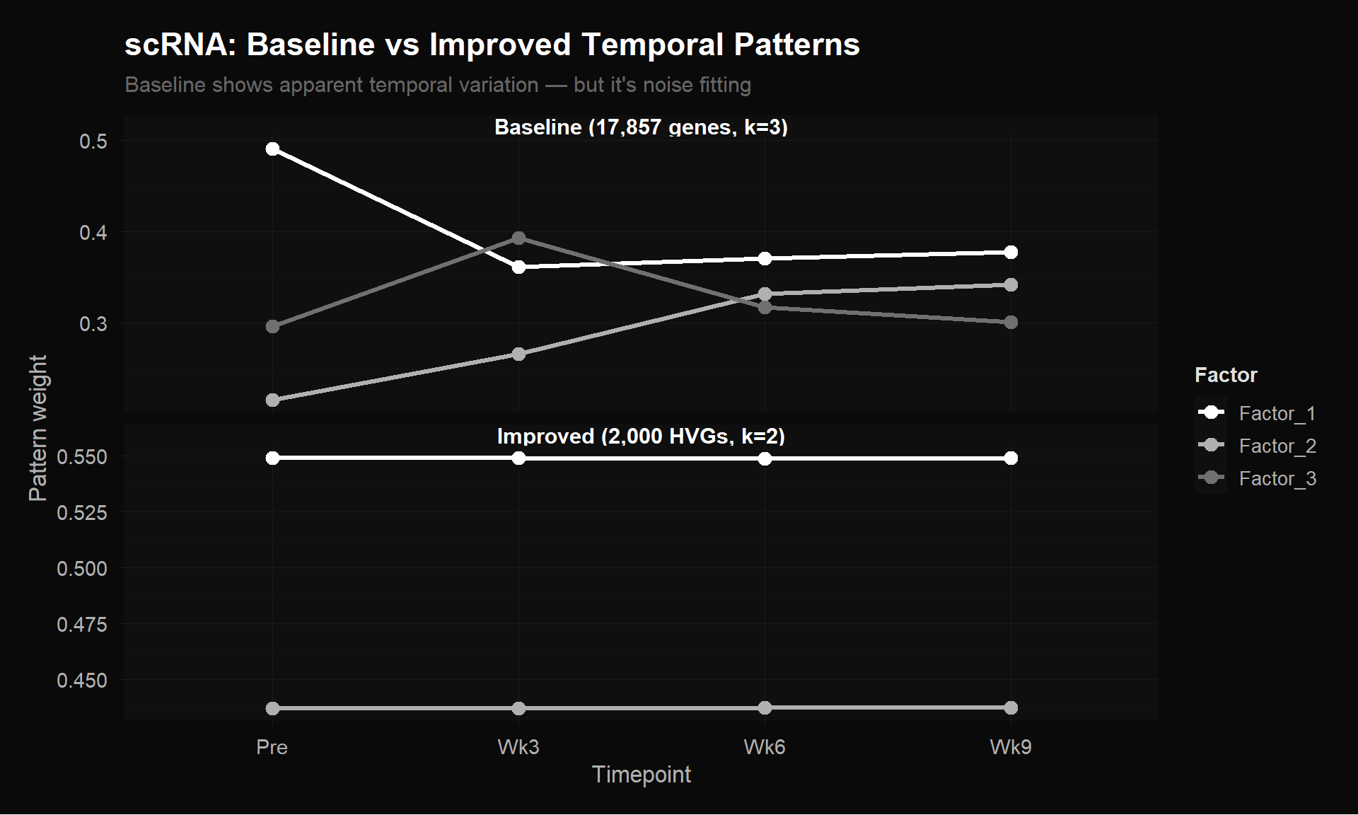

The baseline (top panel) appears to show temporal variation — factors crossing and diverging. But this is noise fitting, not biology. Ethan’s 17,857-gene matrix includes thousands of non-variable genes that add random structure, and the double-log transformation distorts relative magnitudes. MEGPath is fitting this noise.

The improved matrix (bottom, flat lines) is being honest: there simply isn’t temporal signal in pseudobulk averages of 2,000 properly-normalized HVGs. The baseline “patterns” are artifacts of bad preprocessing — they look like signal but carry no biological meaning.

Lesson: Lower error + flat patterns is more trustworthy than higher error + dramatic patterns. The apparent structure in the baseline is noise that MEGPath can partially but not fully fit (hence the 2x higher error).

5b. TCR Comparison

Code

H_tcr_base <- results$tcr_baseline_k3$H
h_tbase_df <- melt(H_tcr_base)
colnames(h_tbase_df) <- c("Factor", "Timepoint", "Weight")
h_tbase_df$Timepoint <- factor(h_tbase_df$Timepoint, levels = timepoints)
h_tbase_df$Matrix <- "Baseline (2,541 clonotypes, k=3)"

h_tbio_df <- h_tcr  # already built above
h_tbio_df$Matrix <- "Bio Filter C (416 clonotypes, k=3)"

h_tcompare <- rbind(h_tbase_df, h_tbio_df)

ggplot(h_tcompare, aes(x = Timepoint, y = Weight, group = Factor, color = Factor)) +
  geom_line(linewidth = 1.2) +
  geom_point(size = 3) +
  facet_wrap(~Matrix, ncol = 1, scales = "free_y") +
  scale_color_donq() +
  labs(title = "TCR: Baseline vs Bio-Filtered Temporal Patterns (k=3)",
       subtitle = "Filter C focuses on treatment-responsive clonotypes",
       y = "Pattern weight") +
  theme_donq()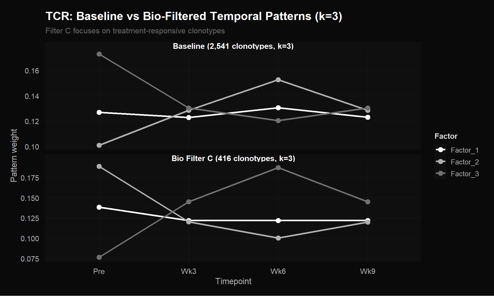

Code

H_tcr_base2 <- results$tcr_baseline_k2$H
h_tbase2_df <- melt(H_tcr_base2)
colnames(h_tbase2_df) <- c("Factor", "Timepoint", "Weight")
h_tbase2_df$Timepoint <- factor(h_tbase2_df$Timepoint, levels = timepoints)
h_tbase2_df$Matrix <- "Baseline (2,541 clonotypes, k=2)"

h_tbio2_df <- h_tcr2  # already built above
h_tbio2_df$Matrix <- "Bio Filter C (416 clonotypes, k=2)"

h_tcompare2 <- rbind(h_tbase2_df, h_tbio2_df)

ggplot(h_tcompare2, aes(x = Timepoint, y = Weight, group = Factor, color = Factor)) +
  geom_line(linewidth = 1.2) +
  geom_point(size = 3) +
  facet_wrap(~Matrix, ncol = 1, scales = "free_y") +
  scale_color_donq() +
  labs(title = "TCR: Baseline vs Bio-Filtered Temporal Patterns (k=2)",
       subtitle = "Same expansion-vs-contraction dichotomy, sharper after filtering",
       y = "Pattern weight") +
  theme_donq()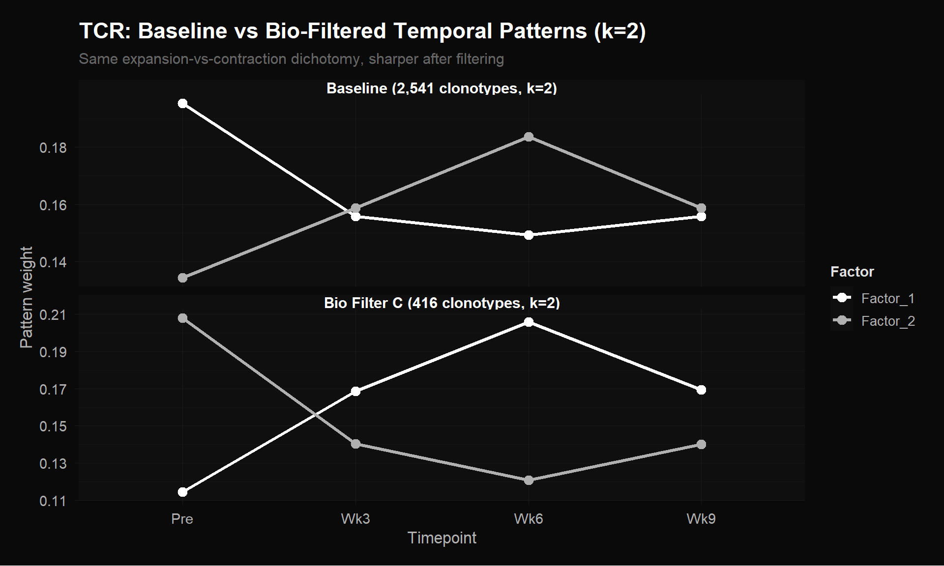

At k=3, the baseline (top panel, 2,541 clonotypes) shows weak, compressed patterns — all three factors hover between 0.10 and 0.17 with mild variation. The ~2,100 single-timepoint clonotypes (96% zeros) act as dead weight, washing out the signal from the ~400 biologically relevant ones. The bio-filtered version (bottom, 416 clonotypes) has much wider separation between factors (range 0.077–0.189) and sharper temporal contrasts. The three distinct programs (stable, contracting, expanding) are clearly resolved.

At k=2, the same pattern holds: the baseline shows a mild crossover, but the bio-filtered version amplifies it into a clean X with wider dynamic range. Both baselines (k=2: LAD/element = 0.00202, k=3: 0.00199) give nearly identical error, suggesting k=2 already captures the dominant structure in the unfiltered data.

6. Conclusions

Code

cat("=== Key Findings ===\n\n")

=== Key Findings ===

Code

cat("1. TCR NMF works: Factor 3 peaks at week 6, independently recovering\n")

1. TCR NMF works: Factor 3 peaks at week 6, independently recovering

Code

cat("   the paper's key finding about CX3CR1+ expansion timing.\n")

   the paper's key finding about CX3CR1+ expansion timing.

Code

cat("   All 6 known treatment-responsive clonotypes assigned to Factor 3.\n\n")

   All 6 known treatment-responsive clonotypes assigned to Factor 3.

Code

cat("2. scRNA pseudobulk NMF does NOT work: flat H matrices = no temporal\n")

2. scRNA pseudobulk NMF does NOT work: flat H matrices = no temporal

Code

cat("   signal at this resolution. Need cluster-level pseudobulk\n")

   signal at this resolution. Need cluster-level pseudobulk

Code

cat("   (genes × [timepoint × cluster]) to preserve cell-type variation.\n\n")

   (genes × [timepoint × cluster]) to preserve cell-type variation.

Code

cat("3. Preprocessing matters more than the algorithm:\n")

3. Preprocessing matters more than the algorithm:

Code

cat("   - Feature selection (17,857 → 2,000 genes): 47% error reduction\n")

   - Feature selection (17,857 → 2,000 genes): 47% error reduction

Code

cat("   - Biological filtering (2,541 → 416 clonotypes): cleaner dynamics\n")

   - Biological filtering (2,541 → 416 clonotypes): cleaner dynamics

Code

cat("   - Both changes make runs 6-10x faster\n\n")

   - Both changes make runs 6-10x faster

Code

cat("4. Baseline 'patterns' are noise: the apparent temporal variation in\n")

4. Baseline 'patterns' are noise: the apparent temporal variation in

Code

cat("   Ethan's 17,857-gene baseline is artifact from noise genes + double-log.\n")

   Ethan's 17,857-gene baseline is artifact from noise genes + double-log.

Code

cat("   Lower error + flat patterns > higher error + fake patterns.\n\n")

   Lower error + flat patterns > higher error + fake patterns.

Code

cat("=== Next Steps ===\n\n")

=== Next Steps ===

Code

cat("1. Build cluster-level scRNA matrix: genes × (timepoint × cluster)\n")

1. Build cluster-level scRNA matrix: genes × (timepoint × cluster)

Code

cat("   to recover temporal signal from cell-type-specific changes.\n\n")

   to recover temporal signal from cell-type-specific changes.

Code

cat("2. Explore MEGPath constraint feature: fix one pattern to the known\n")

2. Explore MEGPath constraint feature: fix one pattern to the known

Code

cat("   CX3CR1 expansion trajectory and let NMF find the rest.\n\n")

   CX3CR1 expansion trajectory and let NMF find the rest.

Code

cat("3. Link TCR Factor 3 clonotypes back to scRNA clusters: which\n")

3. Link TCR Factor 3 clonotypes back to scRNA clusters: which

Code

cat("   transcriptional programs do the expanding clonotypes express?\n")

   transcriptional programs do the expanding clonotypes express?