Code
library(Seurat)
library(NMF)
library(ggplot2)
library(dplyr)
library(reshape2)

source("theme_donq.R")Systematic evaluation of preprocessing choices and their impact on reconstruction error
Script 01 reproduced Ethan’s preprocessing pipeline exactly and identified four issues:
Double log-normalization — AverageExpression(slot="data") returns values that are already log-normalized per cell. Ethan then ran NormalizeData("LogNormalize") on those averages, applying log1p() a second time. This compresses the dynamic range: a gene with true expression 100 vs 10 (10x difference) becomes ~1.8 vs ~1.4 after double-log (~1.3x difference). NMF can’t distinguish biologically meaningful differences from noise when everything is squished together.
RNA assay instead of SCT — The Seurat object contains two assays: RNA (basic log-normalization) and SCT (SCTransform, variance-stabilized). Ethan used RNA, likely because it’s the Seurat default and most tutorials use it.
Averaging in log space — When you average already-log-transformed values, you get the geometric mean, not the arithmetic mean. This systematically underestimates highly-expressed genes.
No feature selection — All 17,857 genes were included. Most genes in scRNA-seq are either not expressed (zeros), expressed at constant levels (housekeeping), or too noisy to be informative. Including them forces NMF to waste factor capacity fitting noise.
This script changes one thing at a time so we can attribute error reduction to specific preprocessing decisions rather than changing everything at once and not knowing what mattered. Every variant is run through the same R NMF algorithm (Lee multiplicative updates, k=2 and k=3, 10 random starts) so errors are directly comparable.
We use LAD (Least Absolute Deviation = sum|V - WH|) as our error metric because that’s what MEGPath optimizes. However, R’s Lee algorithm actually optimizes Frobenius (squared error), so we’re measuring LAD on a solution that wasn’t optimized for LAD. The absolute numbers will differ from MEGPath, but the relative ranking between preprocessing approaches should hold — a cleaner input matrix helps any NMF algorithm.
Additionally, LAD is scale-dependent. A matrix with values in [0, 560] will have larger LAD than a matrix with values in [0, 6] simply because the numbers are bigger. We address this in the normalized comparison section at the end.
NMF decomposes V (n genes x p timepoints) into W (n x k) and H (k x p). Our pseudobulk matrix has only p = 4 columns (Pre, Wk3, Wk6, Wk9), and the rank k cannot meaningfully exceed the smallest matrix dimension. Here’s why:
This is a fundamental limitation of the pseudobulk approach. Averaging all cells into 4 timepoint columns leaves very little room for NMF to find structure. A more granular matrix (e.g., timepoint x cluster = 4 x 13 = 52 columns) would allow higher ranks and potentially richer factor discovery, but requires more careful construction.
library(Seurat)
library(NMF)
library(ggplot2)
library(dplyr)
library(reshape2)
source("theme_donq.R")sobj <- readRDS("NMF Research Data/Copy of Ito_MQ_scRNAseq_sct(1).rds")
cat("Cells:", ncol(sobj), "| Genes:", nrow(sobj), "\n")Cells: 4876 | Genes: 17857 cat("Assays:", paste(Assays(sobj), collapse = ", "), "\n")Assays: RNA, SCT cat("Default assay:", DefaultAssay(sobj), "\n")Default assay: RNA # Reusable function: compute NMF errors for a matrix at given ranks
# Returns a data frame with LAD, Frobenius, and normalized LAD (after [0,1] scaling)
compute_errors <- function(mat, label, ranks = 2:3, nrun = 10) {
# Remove all-zero rows (NMF can't factor zeros meaningfully)
mat <- mat[rowSums(mat) > 0, , drop = FALSE]
# Floor negatives to 0 (SCT Pearson residuals can be slightly negative)
mat <- pmax(mat, 0)
# Remove any new all-zero rows created by flooring
mat <- mat[rowSums(mat) > 0, , drop = FALSE]
results <- list()
for (k in ranks) {
fit <- nmf(mat, rank = k, method = "lee", seed = "random",
nrun = nrun, .opt = "vp2")
residual <- mat - fitted(fit)
frob <- sqrt(sum(residual^2))
lad <- sum(abs(residual))
n_elem <- length(residual)
# Normalized LAD: scale matrix to [0,1] and recompute
mat_norm <- mat / max(mat)
fitted_norm <- fitted(fit) / max(mat)
lad_norm <- sum(abs(mat_norm - fitted_norm))
cat(sprintf("[%s] k=%d: LAD=%.2f, LAD_norm=%.4f, Frobenius=%.2f, Rows=%d\n",
label, k, lad, lad_norm / n_elem, frob, nrow(mat)))
results[[length(results) + 1]] <- data.frame(
label = label, rank = k,
frobenius = frob, lad = lad,
lad_norm = lad_norm,
nmae = lad_norm / n_elem,
n_rows = nrow(mat), n_elements = n_elem,
stringsAsFactors = FALSE
)
}
bind_rows(results)
}# Recompute baselines using our updated error function (which includes NMAE)
# rather than loading from Script 01 (which used an older function without NMAE)
cat("Loading Ethan's CSVs to recompute baselines with normalized error...\n")Loading Ethan's CSVs to recompute baselines with normalized error...dense_raw <- as.matrix(read.csv("NMF Research Data/Data (scRNA, TCR)/dense_data.csv",
header = FALSE))
dense_log <- as.matrix(read.csv("NMF Research Data/Data (scRNA, TCR)/dense_dataLT.csv",
header = FALSE))
tcr_freq <- as.matrix(read.csv("NMF Research Data/Data (scRNA, TCR)/tcr_expansion.csv",
header = FALSE))
colnames(dense_raw) <- colnames(dense_log) <- c("Pre", "Wk3", "Wk6", "Wk9")
colnames(tcr_freq) <- c("Pre", "Wk3", "Wk6", "Wk9")
cat(sprintf("dense_data.csv: %d x %d, range [%.2f, %.2f]\n",
nrow(dense_raw), ncol(dense_raw), min(dense_raw), max(dense_raw)))dense_data.csv: 17857 x 4, range [0.00, 560.93]cat(sprintf("dense_dataLT.csv: %d x %d, range [%.2f, %.2f]\n",
nrow(dense_log), ncol(dense_log), min(dense_log), max(dense_log)))dense_dataLT.csv: 17857 x 4, range [0.00, 6.33]cat(sprintf("tcr_expansion.csv: %d x %d, range [%.2f, %.2f]\n",
nrow(tcr_freq), ncol(tcr_freq), min(tcr_freq), max(tcr_freq)))tcr_expansion.csv: 2541 x 4, range [0.00, 12.05]cat("=== Recomputing Baseline Errors (with NMAE) ===\n\n")=== Recomputing Baseline Errors (with NMAE) ===baseline_raw <- compute_errors(dense_raw, "scRNA raw")
Runs: |
Runs: |                                                  |   0%
Runs: |
Runs: |==================================================| 100%
System time:
   user  system elapsed
   2.65    0.05    6.70
[scRNA raw] k=2: LAD=2402.82, LAD_norm=0.0001, Frobenius=44.58, Rows=17759
Runs: |
Runs: |                                                  |   0%
Runs: |
Runs: |==================================================| 100%
System time:
   user  system elapsed
   2.59    0.00    8.18
[scRNA raw] k=3: LAD=1340.06, LAD_norm=0.0000, Frobenius=20.85, Rows=17759baseline_log <- compute_errors(dense_log, "scRNA log")
Runs: |
Runs: |                                                  |   0%
Runs: |
Runs: |==================================================| 100%
System time:
   user  system elapsed
   2.53    0.00    6.97
[scRNA log] k=2: LAD=1073.09, LAD_norm=0.0024, Frobenius=7.71, Rows=17759
Runs: |
Runs: |                                                  |   0%
Runs: |
Runs: |==================================================| 100%
System time:
   user  system elapsed
   2.58    0.01    9.15
[scRNA log] k=3: LAD=543.23, LAD_norm=0.0012, Frobenius=3.94, Rows=17759baseline_tcr <- compute_errors(tcr_freq, "TCR freq")
Runs: |
Runs: |                                                  |   0%
Runs: |
Runs: |==================================================| 100%
System time:
   user  system elapsed
   2.64    0.00    4.86
[TCR freq] k=2: LAD=298.40, LAD_norm=0.0024, Frobenius=4.86, Rows=2541
Runs: |
Runs: |                                                  |   0%
Runs: |
Runs: |==================================================| 100%
System time:
   user  system elapsed
   2.47    0.08    5.11
[TCR freq] k=3: LAD=186.99, LAD_norm=0.0015, Frobenius=3.18, Rows=2541baseline <- bind_rows(baseline_raw, baseline_log, baseline_tcr)
print(as.data.frame(baseline)) label rank frobenius lad lad_norm nmae n_rows n_elements
1 scRNA raw 2 44.576401 2402.8158 4.283653 6.030257e-05 17759 71036
2 scRNA raw 3 20.851860 1340.0597 2.389010 3.363097e-05 17759 71036
3 scRNA log 2 7.707395 1073.0888 169.487574 2.385939e-03 17759 71036
4 scRNA log 3 3.943797 543.2310 85.799895 1.207837e-03 17759 71036
5 TCR freq 2 4.856518 298.4024 24.767396 2.436777e-03 2541 10164
6 TCR freq 3 3.184668 186.9888 15.520073 1.526965e-03 2541 10164Before running the fixes, here’s what the two assays in this Seurat object actually contain. This matters for understanding why each fix exists.
The default Seurat normalization pipeline (NormalizeData):
log1p(): log(1 + x)Problem: This assumes every gene has the same variance characteristics. In reality, lowly-expressed genes have high variance from sampling noise (a gene detected in 2 vs 0 cells looks like a huge change), while highly-expressed genes have low relative variance. The log transform partially addresses this but doesn’t fully correct it.
A more statistically principled approach:
Result: Variance is stabilized across expression levels. A lowly-expressed immune receptor and a highly-expressed housekeeping gene are on a comparable scale. This prevents NMF from being dominated by a few high-count genes.
Caveat for NMF: SCT values can be negative (Pearson residuals below expected). NMF requires non-negative input, so we floor negatives to zero. This is a minor data loss — in our data, very few values are negative.
How do we know the RNA data slot contains log1p(count / total * 10000)? Because that’s what Seurat’s NormalizeData("LogNormalize") computes by definition. But we can verify it directly by pulling a single cell, taking its raw count for a gene, manually computing the formula, and checking it matches the stored data value.
This matters because Ethan’s double-log bug depends on the data slot already being log-transformed. If we’re wrong about what’s in the data slot, our entire analysis of his preprocessing error would be wrong.
DefaultAssay(sobj) <- "RNA"

# Pick a cell and a gene with a non-zero count
counts_mat <- GetAssayData(sobj, layer = "counts")
data_mat <- GetAssayData(sobj, layer = "data")

# Find a gene-cell pair with a decent count value
# Use the first cell and find a gene with count > 10
cell_idx <- 1
cell_name <- colnames(counts_mat)[cell_idx]
gene_counts <- counts_mat[, cell_idx]
gene_idx <- which(gene_counts > 10)[1]
gene_name <- names(gene_idx)

raw_count <- counts_mat[gene_name, cell_name]
stored_data <- data_mat[gene_name, cell_name]

# Manually compute what NormalizeData("LogNormalize") should produce
total_counts <- sum(counts_mat[, cell_name])
manual_calc <- log1p(raw_count / total_counts * 10000)

cat("=== Sanity Check: RNA data slot = log1p(count / total * 10000) ===\n\n")
=== Sanity Check: RNA data slot = log1p(count / total * 10000) ===cat(sprintf("Cell: %s\n", cell_name))Cell: MQpool1_RS-03742653_AAACCTGTCGCGTTTC-1cat(sprintf("Gene: %s\n", gene_name))Gene: MALAT1cat(sprintf("Raw count: %d\n", raw_count))Raw count: 44cat(sprintf("Total counts in cell: %d\n", total_counts))Total counts in cell: 582cat(sprintf("\nManual calculation: log1p(%d / %d * 10000) = %.10f\n",
raw_count, total_counts, manual_calc))
Manual calculation: log1p(44 / 582 * 10000) = 6.6293814114cat(sprintf("Stored data slot value: %.10f\n", stored_data))Stored data slot value: 6.6293814114cat(sprintf("Difference: %.2e\n",
abs(manual_calc - stored_data)))Difference: 0.00e+00if (abs(manual_calc - stored_data) < 1e-10) {
cat("\nCONFIRMED: RNA data slot contains log1p(count / total * 10000)\n")
cat("This means Ethan's AverageExpression(slot='data') averages LOGGED values.\n")
cat("His subsequent NormalizeData() then logs them AGAIN -> double-log.\n")
} else {
cat("\nWARNING: Values don't match — investigate further.\n")
}
CONFIRMED: RNA data slot contains log1p(count / total * 10000)
This means Ethan's AverageExpression(slot='data') averages LOGGED values.
His subsequent NormalizeData() then logs them AGAIN -> double-log.DefaultAssay(sobj) <- "RNA"
rna_data <- GetAssayData(sobj, layer = "data")
rna_range <- range(rna_data)
DefaultAssay(sobj) <- "SCT"
sct_data <- GetAssayData(sobj, layer = "data")
sct_range <- range(sct_data)
sct_neg <- sum(sct_data < 0)
sct_total <- length(sct_data)
cat("RNA data layer range:", rna_range, "\n")RNA data layer range: 0 7.750948 cat("SCT data layer range:", sct_range, "\n")SCT data layer range: 0 6.023448 cat("SCT negative values:", sct_neg, "of", sct_total,
sprintf("(%.3f%%)\n", 100 * sct_neg / sct_total))SCT negative values: 0 of 74700320 (0.000%)What this fixes: Ethan’s double-log bug, nothing else.
Ethan’s pipeline: AverageExpression(slot="data") → averages already-log-normalized values → NormalizeData() → applies log1p a second time.
Our fix: average the raw counts across cells per timepoint first, then apply log1p once. This gives us properly log-normalized pseudobulk values. Same number of genes (all 17,857), same normalization philosophy — just done correctly.
DefaultAssay(sobj) <- "RNA"

# Average raw counts per timepoint (NOT the log-normalized data slot)
avg_counts <- AverageExpression(sobj, group.by = "HTO_maxID",
                                 assays = "RNA", slot = "counts")$RNA
avg_counts <- as.matrix(avg_counts)
avg_counts <- avg_counts[, c("HashTag1", "HashTag2", "HashTag3", "HashTag4")]
colnames(avg_counts) <- c("Pre", "Wk3", "Wk6", "Wk9")

cat("Averaged raw counts:", nrow(avg_counts), "x", ncol(avg_counts), "\n")
Averaged raw counts: 17857 x 4 cat("Range:", range(avg_counts), "\n")Range: 0 121.5023 # Single log-normalization: log1p(x)
fix1_mat <- log1p(avg_counts)
cat("After log1p:", nrow(fix1_mat), "x", ncol(fix1_mat), "range:", range(fix1_mat), "\n")After log1p: 17857 x 4 range: 0 4.80813 cat("\n")fix1_errors <- compute_errors(fix1_mat, "Fix1: single log")
Runs: |
Runs: |                                                  |   0%
Runs: |
Runs: |==================================================| 100%
System time:
   user  system elapsed
   2.56    0.02    7.25
[Fix1: single log] k=2: LAD=514.37, LAD_norm=0.0015, Frobenius=4.11, Rows=17759
Runs: |
Runs: |                                                  |   0%
Runs: |
Runs: |==================================================| 100%
System time:
   user  system elapsed
   2.57    0.04    9.84
[Fix1: single log] k=3: LAD=213.70, LAD_norm=0.0006, Frobenius=1.99, Rows=17759What this fixes: The normalization method only. Still uses all genes.
Instead of RNA’s simple log-normalization, use SCT’s variance-stabilized values. If the assay choice alone matters, this should show improvement over baseline.
SCT contains 15,320 genes (vs RNA’s 17,857) because SCTransform drops genes it can’t model reliably — genes with too few counts or too little variation. This is actually a feature: those dropped genes were uninformative anyway.
DefaultAssay(sobj) <- "SCT"

# Average SCT-normalized values per timepoint
avg_sct <- AverageExpression(sobj, group.by = "HTO_maxID",
                              assays = "SCT", slot = "data")$SCT
avg_sct <- as.matrix(avg_sct)
avg_sct <- avg_sct[, c("HashTag1", "HashTag2", "HashTag3", "HashTag4")]
colnames(avg_sct) <- c("Pre", "Wk3", "Wk6", "Wk9")

cat("SCT averaged:", nrow(avg_sct), "x", ncol(avg_sct), "\n")
SCT averaged: 15320 x 4 cat("Range:", range(avg_sct), "\n")Range: 0 122.1817 cat("Negatives:", sum(avg_sct < 0), "\n")Negatives: 0 # Floor negatives to 0 for NMF non-negativity requirement
fix2_mat <- pmax(avg_sct, 0)
cat("After floor:", range(fix2_mat), "\n")After floor: 0 122.1817 cat("\n")fix2_errors <- compute_errors(fix2_mat, "Fix2: SCT assay")
Runs: |
Runs: |                                                  |   0%
Runs: |
Runs: |==================================================| 100%
System time:
   user  system elapsed
   2.64    0.01    7.27
[Fix2: SCT assay] k=2: LAD=880.68, LAD_norm=0.0001, Frobenius=18.40, Rows=15320
Runs: |
Runs: |                                                  |   0%
Runs: |
Runs: |==================================================| 100%
System time:
   user  system elapsed
   2.75    0.02    8.20
[Fix2: SCT assay] k=3: LAD=456.91, LAD_norm=0.0001, Frobenius=11.10, Rows=15320Before running Fixes 3-5, we need to understand why feature selection matters for NMF.
Of the 17,857 genes in this dataset:
NMF with rank k=3 has only 3 factors to explain the entire matrix. With 17,857 rows, each factor is responsible for ~6,000 genes. Most of those genes are flat noise, so the factors end up as blurry compromises between signal and noise. By filtering to the top 2,000 highly variable genes (HVGs), NMF can focus its limited factor capacity on genes that actually change across timepoints.
Seurat’s FindVariableFeatures() (or SCTransform’s built-in variance estimation) ranks genes by how much their observed variance exceeds what you’d expect given their mean expression level. The ranking roughly looks like:
The number 2,000 is a field convention, not a theoretically derived threshold. It comes from Seurat’s default FindVariableFeatures(nfeatures = 2000). The Satija lab found empirically that ~2,000 genes captures enough biological variation for clustering and dimensionality reduction across most scRNA-seq datasets. Nearly every published single-cell paper uses 2,000-3,000 HVGs.
We test whether this default is optimal in the Gene Count Sweep section below, where we run NMF at 500, 1000, 2000, 3000, and 5000 genes to find the sweet spot.
DefaultAssay(sobj) <- "SCT"
hvgs <- VariableFeatures(sobj)
cat("Pre-computed HVGs from SCTransform:", length(hvgs), "\n")
Pre-computed HVGs from SCTransform: 3000 if (length(hvgs) < 2000) {
sobj <- FindVariableFeatures(sobj, nfeatures = 2000)
hvgs <- VariableFeatures(sobj)
}
hvgs_2k <- head(hvgs, 2000)
cat("Using top", length(hvgs_2k), "HVGs for Fixes 3-5\n")Using top 2000 HVGs for Fixes 3-5We have 16 genes of known biological importance from the source paper (Abdelfatah et al. 2023). These include CX3CR1+ effector markers (GZMB, PRF1, NKG7), early activation markers (GZMK, CXCR3), naive/memory markers (TCF7, SELL), exhaustion markers (LAG3, TIGIT, PDCD1, HAVCR2), and a proliferation marker (MKI67). We need to verify our HVG cutoff captures them.
bio_genes <- c("CX3CR1", "GZMB", "GZMH", "PRF1", "NKG7", "CCL4", "CCL5",
               "GZMK", "CXCR3", "TCF7", "SELL", "LAG3", "TIGIT", "PDCD1",
               "HAVCR2", "MKI67")

in_hvg <- bio_genes %in% hvgs_2k
cat("Key biology genes in top 2k HVGs:", sum(in_hvg), "of", length(bio_genes), "\n")
Key biology genes in top 2k HVGs: 14 of 16 cat("Captured:", paste(bio_genes[in_hvg], collapse = ", "), "\n")Captured: CX3CR1, GZMB, GZMH, PRF1, NKG7, CCL4, CCL5, GZMK, CXCR3, TCF7, SELL, LAG3, TIGIT, MKI67 cat("Missing:", paste(bio_genes[!in_hvg], collapse = ", "), "\n\n")Missing: PDCD1, HAVCR2 # Where do the missing genes rank?
missing <- bio_genes[!in_hvg]
if (length(missing) > 0) {
for (g in missing) {
rank_pos <- which(hvgs == g)
if (length(rank_pos) > 0) {
cat(sprintf(" %s: ranked #%d out of %d HVGs\n", g, rank_pos, length(hvgs)))
} else {
cat(sprintf(" %s: not in HVG list at all (very low variance)\n", g))
}
}
} PDCD1: ranked #2594 out of 3000 HVGs
HAVCR2: not in HVG list at all (very low variance)What this fixes: Gene count only. Uses Ethan’s exact normalization path (RNA data slot = single log-normalized averages) but restricted to top 2,000 HVGs. This isolates the effect of removing noise genes from the effect of changing normalization.
DefaultAssay(sobj) <- "RNA"

hvgs_available <- hvgs_2k[hvgs_2k %in% rownames(sobj)]

avg_rna_hvg <- AverageExpression(sobj, group.by = "HTO_maxID",
                                  assays = "RNA", slot = "data",
                                  features = hvgs_available)$RNA
avg_rna_hvg <- as.matrix(avg_rna_hvg)
avg_rna_hvg <- avg_rna_hvg[, c("HashTag1", "HashTag2", "HashTag3", "HashTag4")]
colnames(avg_rna_hvg) <- c("Pre", "Wk3", "Wk6", "Wk9")

cat("Fix3 (Ethan's norm + HVGs):", nrow(avg_rna_hvg), "x", ncol(avg_rna_hvg), "\n")
Fix3 (Ethan's norm + HVGs): 2000 x 4 cat("Range:", range(avg_rna_hvg), "\n")Range: 0 137.2963 cat("\n")fix3_errors <- compute_errors(avg_rna_hvg, "Fix3: RNA + 2k HVGs")
Runs: |
Runs: |                                                  |   0%
Runs: |
Runs: |==================================================| 100%
System time:
   user  system elapsed
   2.57    0.00    4.92
[Fix3: RNA + 2k HVGs] k=2: LAD=700.56, LAD_norm=0.0006, Frobenius=38.19, Rows=2000
Runs: |
Runs: |                                                  |   0%
Runs: |
Runs: |==================================================| 100%
System time:
   user  system elapsed
   2.52    0.01    5.28
[Fix3: RNA + 2k HVGs] k=3: LAD=326.97, LAD_norm=0.0003, Frobenius=13.87, Rows=2000What this fixes: Both normalization and gene selection. Uses SCTransform variance-stabilized values restricted to the 2,000 most informative genes. The idea: SCT puts all genes on a comparable scale (no single gene dominates the factorization) AND HVG filtering removes genes that don’t vary across timepoints. We expect these improvements to compound.
DefaultAssay(sobj) <- "SCT"

hvgs_in_sct <- hvgs_2k[hvgs_2k %in% rownames(sobj)]

avg_sct_hvg <- AverageExpression(sobj, group.by = "HTO_maxID",
                                  assays = "SCT", slot = "data",
                                  features = hvgs_in_sct)$SCT
avg_sct_hvg <- as.matrix(avg_sct_hvg)
avg_sct_hvg <- avg_sct_hvg[, c("HashTag1", "HashTag2", "HashTag3", "HashTag4")]
colnames(avg_sct_hvg) <- c("Pre", "Wk3", "Wk6", "Wk9")

cat("Fix4 (SCT + HVGs):", nrow(avg_sct_hvg), "x", ncol(avg_sct_hvg), "\n")
Fix4 (SCT + HVGs): 2000 x 4 cat("Range:", range(avg_sct_hvg), "\n")Range: 0 48.22649 cat("Negatives:", sum(avg_sct_hvg < 0), "\n")Negatives: 0 fix4_mat <- pmax(avg_sct_hvg, 0)
cat("\n")fix4_errors <- compute_errors(fix4_mat, "Fix4: SCT + 2k HVGs")
Runs: |
Runs: |                                                  |   0%
Runs: |
Runs: |==================================================| 100%
System time:
   user  system elapsed
   2.64    0.02    5.08
[Fix4: SCT + 2k HVGs] k=2: LAD=252.80, LAD_norm=0.0007, Frobenius=14.00, Rows=2000
Runs: |
Runs: |                                                  |   0%
Runs: |
Runs: |==================================================| 100%
System time:
   user  system elapsed
   3.06    0.01    5.65
[Fix4: SCT + 2k HVGs] k=3: LAD=110.11, LAD_norm=0.0003, Frobenius=5.25, Rows=2000What this fixes: Tests whether we should normalize at all before MEGPath.
MEGPath normalizes every input to [0,1] internally before running NMF. So if we feed it log1p(counts), MEGPath sees normalize_to_01(log(counts)). If we feed it raw counts, MEGPath sees normalize_to_01(counts). The log transform might add information (compressing the dynamic range to help NMF), or it might be redundant since MEGPath handles scaling internally.
This fix gives MEGPath the rawest informative data: averaged raw counts for only the top 2,000 HVGs. No log, no normalization — just the arithmetic mean of counts per gene per timepoint.
DefaultAssay(sobj) <- "RNA"

avg_counts_hvg <- AverageExpression(sobj, group.by = "HTO_maxID",
                                     assays = "RNA", slot = "counts",
                                     features = hvgs_available)$RNA
avg_counts_hvg <- as.matrix(avg_counts_hvg)
avg_counts_hvg <- avg_counts_hvg[, c("HashTag1", "HashTag2", "HashTag3", "HashTag4")]
colnames(avg_counts_hvg) <- c("Pre", "Wk3", "Wk6", "Wk9")

cat("Fix5 (raw counts + HVGs):", nrow(avg_counts_hvg), "x", ncol(avg_counts_hvg), "\n")
Fix5 (raw counts + HVGs): 2000 x 4 cat("Range:", range(avg_counts_hvg), "\n")Range: 0 61.58259 cat("\n")fix5_errors <- compute_errors(avg_counts_hvg, "Fix5: counts + 2k HVGs")
Runs: |
Runs: |                                                  |   0%
Runs: |
Runs: |==================================================| 100%
System time:
   user  system elapsed
   2.77    0.06    5.17
[Fix5: counts + 2k HVGs] k=2: LAD=318.48, LAD_norm=0.0006, Frobenius=16.26, Rows=2000
Runs: |
Runs: |                                                  |   0%
Runs: |
Runs: |==================================================| 100%
System time:
   user  system elapsed
   2.49    0.02    5.22
[Fix5: counts + 2k HVGs] k=3: LAD=115.72, LAD_norm=0.0002, Frobenius=5.69, Rows=2000The 2,000 HVG cutoff is a convention, not an optimization. Here we test whether a different number of genes would perform better for NMF specifically. We run NMF on SCT + HVGs (our best normalization from Fix 4) at gene counts of 500, 1000, 2000, 3000, and 5000.
Tradeoff: Fewer genes → less noise, but risk losing biology. More genes → more coverage, but NMF wastes capacity on flat genes. We also check biology gene coverage at each cutoff.
# SCT pre-computed 3000 HVGs. For 5000 we need to recompute.
DefaultAssay(sobj) <- "SCT"
if (length(hvgs) < 5000) {
  cat("Recomputing HVGs with nfeatures=5000 for sweep...\n")
  sobj <- FindVariableFeatures(sobj, nfeatures = 5000)
  hvgs_extended <- VariableFeatures(sobj)
  cat(sprintf("Extended HVG list: %d genes\n", length(hvgs_extended)))
} else {
  hvgs_extended <- hvgs
}
Recomputing HVGs with nfeatures=5000 for sweep...
Extended HVG list: 5000 genesgene_counts <- c(500, 1000, 2000, 3000, 5000)
bio_genes_all <- c("CX3CR1", "GZMB", "GZMH", "PRF1", "NKG7", "CCL4", "CCL5",
"GZMK", "CXCR3", "TCF7", "SELL", "LAG3", "TIGIT", "PDCD1",
"HAVCR2", "MKI67")
sweep_results <- list()
sweep_bio <- list()
for (ng in gene_counts) {
cat(sprintf("\n=== %d genes ===\n", ng))
# Select top N HVGs from extended list
hvg_subset <- head(hvgs_extended, ng)
hvg_in_sct <- hvg_subset[hvg_subset %in% rownames(sobj)]
cat(sprintf("Requested: %d, Available in SCT: %d\n", ng, length(hvg_in_sct)))
# Biology coverage
n_bio <- sum(bio_genes_all %in% hvg_in_sct)
captured <- bio_genes_all[bio_genes_all %in% hvg_in_sct]
missing_bio <- bio_genes_all[!bio_genes_all %in% hvg_in_sct]
cat(sprintf("Biology genes captured: %d / %d\n", n_bio, length(bio_genes_all)))
if (length(missing_bio) > 0) cat("Missing:", paste(missing_bio, collapse = ", "), "\n")
sweep_bio[[as.character(ng)]] <- data.frame(
n_genes = ng, n_bio_captured = n_bio,
missing = paste(missing_bio, collapse = ", "),
stringsAsFactors = FALSE
)
# Build matrix
DefaultAssay(sobj) <- "SCT"
avg_tmp <- AverageExpression(sobj, group.by = "HTO_maxID",
assays = "SCT", slot = "data",
features = hvg_in_sct)$SCT
avg_tmp <- as.matrix(avg_tmp)
avg_tmp <- avg_tmp[, c("HashTag1", "HashTag2", "HashTag3", "HashTag4")]
colnames(avg_tmp) <- c("Pre", "Wk3", "Wk6", "Wk9")
avg_tmp <- pmax(avg_tmp, 0)
# Run NMF
errors_tmp <- compute_errors(avg_tmp, sprintf("SCT + %d HVGs", ng), ranks = 2:3, nrun = 10)
sweep_results[[length(sweep_results) + 1]] <- errors_tmp
}
=== 500 genes ===
Requested: 500, Available in SCT: 500
Biology genes captured: 10 / 16
Missing: CXCR3, TCF7, SELL, TIGIT, PDCD1, HAVCR2
Runs: |
Runs: |                                                  |   0%
Runs: |
Runs: |==================================================| 100%
System time:
   user  system elapsed
   2.47    0.06    4.36
[SCT + 500 HVGs] k=2: LAD=153.78, LAD_norm=0.0016, Frobenius=12.88, Rows=500
Runs: |
Runs: |                                                  |   0%
Runs: |
Runs: |==================================================| 100%
System time:
   user  system elapsed
   2.42    0.03    4.61
[SCT + 500 HVGs] k=3: LAD=53.28, LAD_norm=0.0006, Frobenius=4.10, Rows=500

=== 1000 genes ===
Requested: 1000, Available in SCT: 1000
Biology genes captured: 13 / 16
Missing: TCF7, PDCD1, HAVCR2
Runs: |
Runs: |                                                  |   0%
Runs: |
Runs: |==================================================| 100%
System time:
   user  system elapsed
   2.67    0.00    4.72
[SCT + 1000 HVGs] k=2: LAD=191.97, LAD_norm=0.0010, Frobenius=13.51, Rows=1000
Runs: |
Runs: |                                                  |   0%
Runs: |
Runs: |==================================================| 100%
System time:
   user  system elapsed
   2.50    0.03    4.94
[SCT + 1000 HVGs] k=3: LAD=78.33, LAD_norm=0.0004, Frobenius=4.71, Rows=1000

=== 2000 genes ===
Requested: 2000, Available in SCT: 2000
Biology genes captured: 14 / 16
Missing: PDCD1, HAVCR2
Runs: |
Runs: |                                                  |   0%
Runs: |
Runs: |==================================================| 100%
System time:
   user  system elapsed
   2.45    0.02    4.73
[SCT + 2000 HVGs] k=2: LAD=252.86, LAD_norm=0.0007, Frobenius=14.00, Rows=2000
Runs: |
Runs: |                                                  |   0%
Runs: |
Runs: |==================================================| 100%
System time:
   user  system elapsed
   2.52    0.04    4.98
[SCT + 2000 HVGs] k=3: LAD=98.69, LAD_norm=0.0003, Frobenius=4.85, Rows=2000

=== 3000 genes ===
Requested: 3000, Available in SCT: 3000
Biology genes captured: 15 / 16
Missing: HAVCR2
Runs: |
Runs: |                                                  |   0%
Runs: |
Runs: |==================================================| 100%
System time:
   user  system elapsed
   2.52    0.03    5.00
[SCT + 3000 HVGs] k=2: LAD=304.60, LAD_norm=0.0005, Frobenius=14.30, Rows=3000
Runs: |
Runs: |                                                  |   0%
Runs: |
Runs: |==================================================| 100%
System time:
   user  system elapsed
   2.44    0.07    5.35
[SCT + 3000 HVGs] k=3: LAD=142.55, LAD_norm=0.0002, Frobenius=5.63, Rows=3000

=== 5000 genes ===
Requested: 5000, Available in SCT: 5000
Biology genes captured: 16 / 16
Runs: |
Runs: |                                                  |   0%
Runs: |
Runs: |==================================================| 100%
System time:
   user  system elapsed
   2.47    0.03    5.13
[SCT + 5000 HVGs] k=2: LAD=392.51, LAD_norm=0.0004, Frobenius=14.62, Rows=5000
Runs: |
Runs: |                                                  |   0%
Runs: |
Runs: |==================================================| 100%
System time:
   user  system elapsed
   2.53    0.03    5.49
[SCT + 5000 HVGs] k=3: LAD=159.17, LAD_norm=0.0002, Frobenius=5.14, Rows=5000sweep_errors <- bind_rows(sweep_results)
sweep_bio_df <- bind_rows(sweep_bio)cat("=== Biology Gene Coverage by HVG Cutoff ===\n\n")=== Biology Gene Coverage by HVG Cutoff ===print(as.data.frame(sweep_bio_df)) n_genes n_bio_captured missing
1 500 10 CXCR3, TCF7, SELL, TIGIT, PDCD1, HAVCR2
2 1000 13 TCF7, PDCD1, HAVCR2
3 2000 14 PDCD1, HAVCR2
4 3000 15 HAVCR2
5 5000 16 sweep_plot_data <- sweep_errors |>
mutate(n_genes = as.numeric(gsub("SCT \\+ (\\d+) HVGs", "\\1", label)))
p_sweep <- ggplot(sweep_plot_data, aes(x = n_genes, y = nmae, color = factor(rank))) +
geom_line(linewidth = 1.2) +
geom_point(size = 3) +
scale_color_donq() +
theme_donq() +
scale_x_continuous(breaks = gene_counts) +
labs(
title = "Gene Count Sweep: Normalized Error vs Number of HVGs",
subtitle = "SCT assay | Normalized MAE (LAD on [0,1]-scaled matrix / n_elements)",
x = "Number of Highly Variable Genes",
y = "Normalized MAE",
color = "Rank (k)",
caption = "Lee algorithm, 10 random starts | eigen.io"
)
p_sweep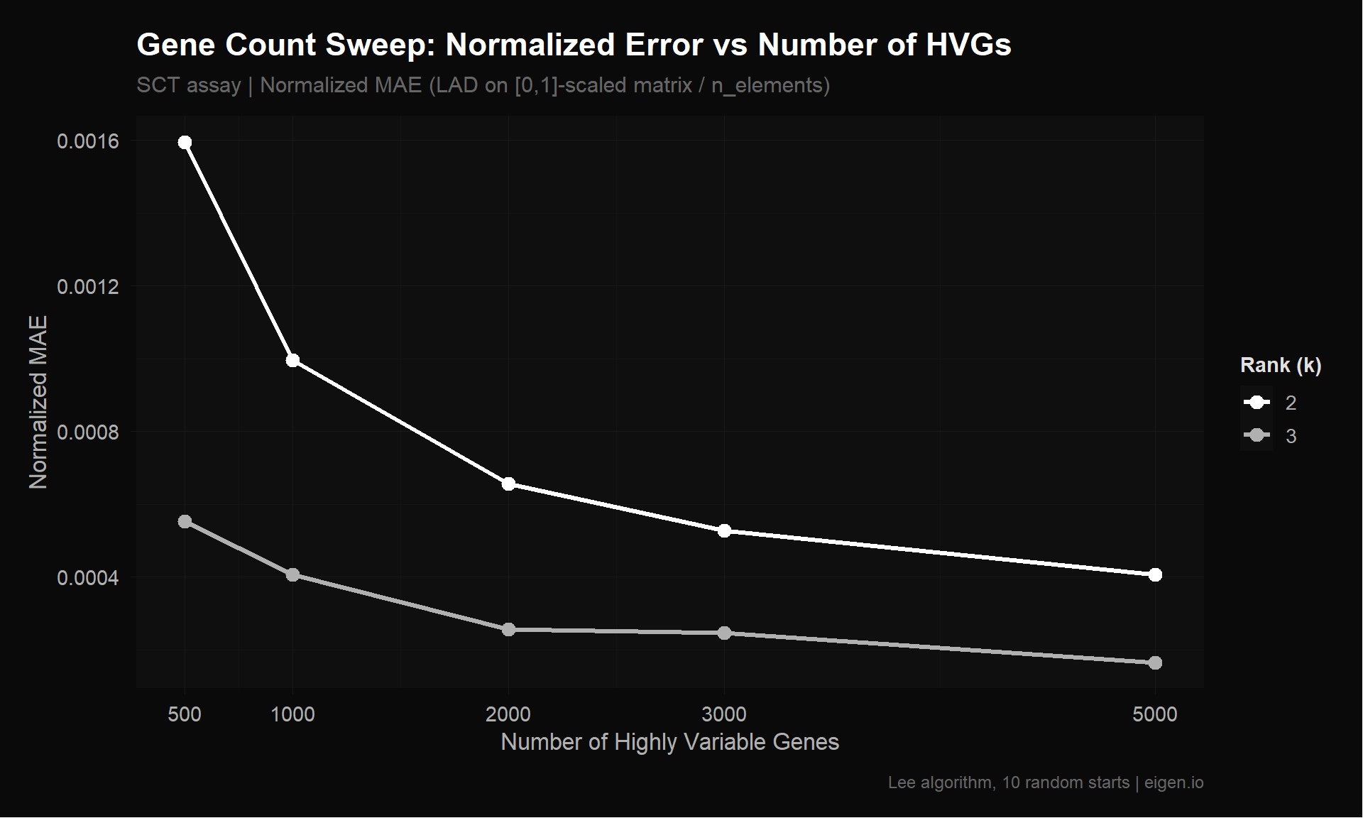
save_donq(p_sweep, "02_gene_sweep.png", width = 10, height = 6)p_sweep_lad <- ggplot(sweep_plot_data, aes(x = n_genes, y = lad, color = factor(rank))) +
geom_line(linewidth = 1.2) +
geom_point(size = 3) +
scale_color_donq() +
theme_donq() +
scale_x_continuous(breaks = gene_counts) +
labs(
title = "Gene Count Sweep: Total LAD vs Number of HVGs",
subtitle = "Total reconstruction error increases with more genes (more to fit)",
x = "Number of Highly Variable Genes",
y = "Least Absolute Deviation (LAD)",
color = "Rank (k)",
caption = "Lee algorithm, 10 random starts | eigen.io"
)
p_sweep_lad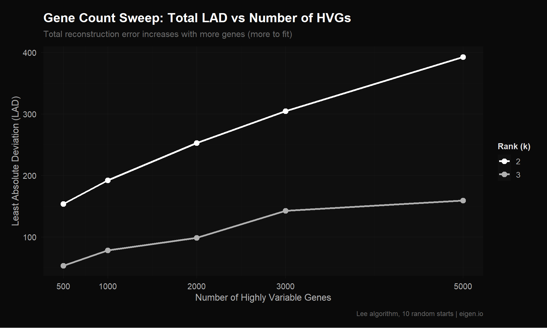
save_donq(p_sweep_lad, "02_gene_sweep_lad.png", width = 10, height = 6)Caution: Raw LAD is not directly comparable across matrices with different value ranges. A matrix with values in [0, 560] will naturally have higher LAD than one in [0, 6] even if the relative fit quality is identical. This is why Ethan’s double-log (which compressed values to [0, 6.33]) appeared to have lower error — the values were smaller, not the fit better.
Within the same matrix (comparing k=2 vs k=3), raw LAD is valid. Across matrices with similar scales (e.g., Fix 4 vs Fix 5, both HVG-filtered), it’s approximately valid.
all_errors <- bind_rows(
  baseline,
  fix1_errors,
  fix2_errors,
  fix3_errors,
  fix4_errors,
  fix5_errors
)

cat("=== All Error Comparisons (raw LAD) ===\n")
=== All Error Comparisons (raw LAD) ===all_errors |>
filter(!grepl("TCR", label)) |>
arrange(rank, lad) |>
select(label, rank, n_rows, lad, frobenius, nmae) |>
as.data.frame() |>
print() label rank n_rows lad frobenius nmae
1 Fix4: SCT + 2k HVGs 2 2000 252.7993 13.999031 6.552398e-04
2 Fix5: counts + 2k HVGs 2 2000 318.4837 16.259852 6.464565e-04
3 Fix1: single log 2 17759 514.3735 4.114701 1.505996e-03
4 Fix3: RNA + 2k HVGs 2 2000 700.5550 38.192316 6.378129e-04
5 Fix2: SCT assay 2 15320 880.6825 18.404199 1.176236e-04
6 scRNA log 2 17759 1073.0888 7.707395 2.385939e-03
7 scRNA raw 2 17759 2402.8158 44.576401 6.030257e-05
8 Fix4: SCT + 2k HVGs 3 2000 110.1084 5.249164 2.853941e-04
9 Fix5: counts + 2k HVGs 3 2000 115.7164 5.693247 2.348805e-04
10 Fix1: single log 3 17759 213.6954 1.994523 6.256630e-04
11 Fix3: RNA + 2k HVGs 3 2000 326.9715 13.872048 2.976877e-04
12 Fix2: SCT assay 3 15320 456.9076 11.104950 6.102440e-05
13 scRNA log 3 17759 543.2310 3.943797 1.207837e-03
14 scRNA raw 3 17759 1340.0597 20.851860 3.363097e-05To fairly compare across matrices with different value ranges, we normalize each matrix to [0, 1] before computing error. This is also what MEGPath does internally — it rescales to [0, 1] first, then runs NMF. So the normalized MAE (NMAE) is the closest proxy we have for how MEGPath will rank these matrices.
cat("=== Normalized MAE (error after [0,1] scaling, per element) ===\n")=== Normalized MAE (error after [0,1] scaling, per element) ===cat("This is the fairest cross-matrix comparison.\n\n")This is the fairest cross-matrix comparison.all_errors |>
filter(!grepl("TCR", label)) |>
arrange(rank, nmae) |>
select(label, rank, n_rows, nmae) |>
as.data.frame() |>
print() label rank n_rows nmae
1 scRNA raw 2 17759 6.030257e-05
2 Fix2: SCT assay 2 15320 1.176236e-04
3 Fix3: RNA + 2k HVGs 2 2000 6.378129e-04
4 Fix5: counts + 2k HVGs 2 2000 6.464565e-04
5 Fix4: SCT + 2k HVGs 2 2000 6.552398e-04
6 Fix1: single log 2 17759 1.505996e-03
7 scRNA log 2 17759 2.385939e-03
8 scRNA raw 3 17759 3.363097e-05
9 Fix2: SCT assay 3 15320 6.102440e-05
10 Fix5: counts + 2k HVGs 3 2000 2.348805e-04
11 Fix4: SCT + 2k HVGs 3 2000 2.853941e-04
12 Fix3: RNA + 2k HVGs 3 2000 2.976877e-04
13 Fix1: single log 3 17759 6.256630e-04
14 scRNA log 3 17759 1.207837e-03cat("\n=== Improvement vs Ethan's Baseline (Normalized MAE) ===\n\n")
=== Improvement vs Ethan's Baseline (Normalized MAE) ===# Use Ethan's double-log (scRNA log) as the baseline — that's what he actually used
for (k in 2:3) {
baseline_best <- all_errors |>
filter(label == "scRNA log", rank == k)
improved <- all_errors |>
filter(!grepl("scRNA|TCR", label), rank == k) |>
arrange(nmae)
cat(sprintf("--- Rank k=%d (baseline NMAE: %.6f from %s) ---\n",
k, baseline_best$nmae[1], baseline_best$label[1]))
for (i in 1:nrow(improved)) {
pct <- 100 * (baseline_best$nmae[1] - improved$nmae[i]) / baseline_best$nmae[1]
cat(sprintf(" %s: NMAE=%.6f (%+.1f%%, %d rows)\n",
improved$label[i], improved$nmae[i], -pct, improved$n_rows[i]))
}
cat("\n")
}--- Rank k=2 (baseline NMAE: 0.002386 from scRNA log) ---
Fix2: SCT assay: NMAE=0.000118 (-95.1%, 15320 rows)
Fix3: RNA + 2k HVGs: NMAE=0.000638 (-73.3%, 2000 rows)
Fix5: counts + 2k HVGs: NMAE=0.000646 (-72.9%, 2000 rows)
Fix4: SCT + 2k HVGs: NMAE=0.000655 (-72.5%, 2000 rows)
Fix1: single log: NMAE=0.001506 (-36.9%, 17759 rows)
--- Rank k=3 (baseline NMAE: 0.001208 from scRNA log) ---
Fix2: SCT assay: NMAE=0.000061 (-94.9%, 15320 rows)
Fix5: counts + 2k HVGs: NMAE=0.000235 (-80.6%, 2000 rows)
Fix4: SCT + 2k HVGs: NMAE=0.000285 (-76.4%, 2000 rows)
Fix3: RNA + 2k HVGs: NMAE=0.000298 (-75.4%, 2000 rows)
Fix1: single log: NMAE=0.000626 (-48.2%, 17759 rows)plot_data <- all_errors |>
filter(!grepl("TCR", label)) |>
mutate(label = factor(label, levels = unique(label)))
p_compare <- ggplot(plot_data, aes(x = label, y = lad, fill = factor(rank))) +
geom_col(position = "dodge", width = 0.7) +
scale_fill_donq() +
theme_donq() +
theme(axis.text.x = element_text(angle = 35, hjust = 1, size = 10)) +
labs(
title = "scRNA NMF Error: Baseline vs Improved Preprocessing",
subtitle = "Raw LAD (sum |V - WH|) — lower is better, but not comparable across different value scales",
x = NULL,
y = "Least Absolute Deviation",
fill = "Rank (k)",
caption = "Lee algorithm, 10 random starts | eigen.io"
)
p_compare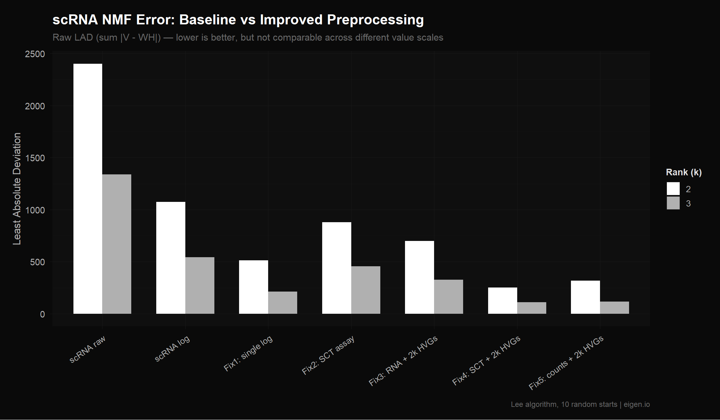
save_donq(p_compare, "02_error_comparison.png", width = 12, height = 7)p_nmae <- ggplot(plot_data, aes(x = label, y = nmae, fill = factor(rank))) +
geom_col(position = "dodge", width = 0.7) +
scale_fill_donq() +
theme_donq() +
theme(axis.text.x = element_text(angle = 35, hjust = 1, size = 10)) +
labs(
title = "scRNA NMF Error: Normalized MAE (Scale-Independent)",
subtitle = "Each matrix scaled to [0,1] before computing error — fair comparison across all variants",
x = NULL,
y = "Normalized MAE",
fill = "Rank (k)",
caption = "Lee algorithm, 10 random starts | eigen.io"
)
p_nmae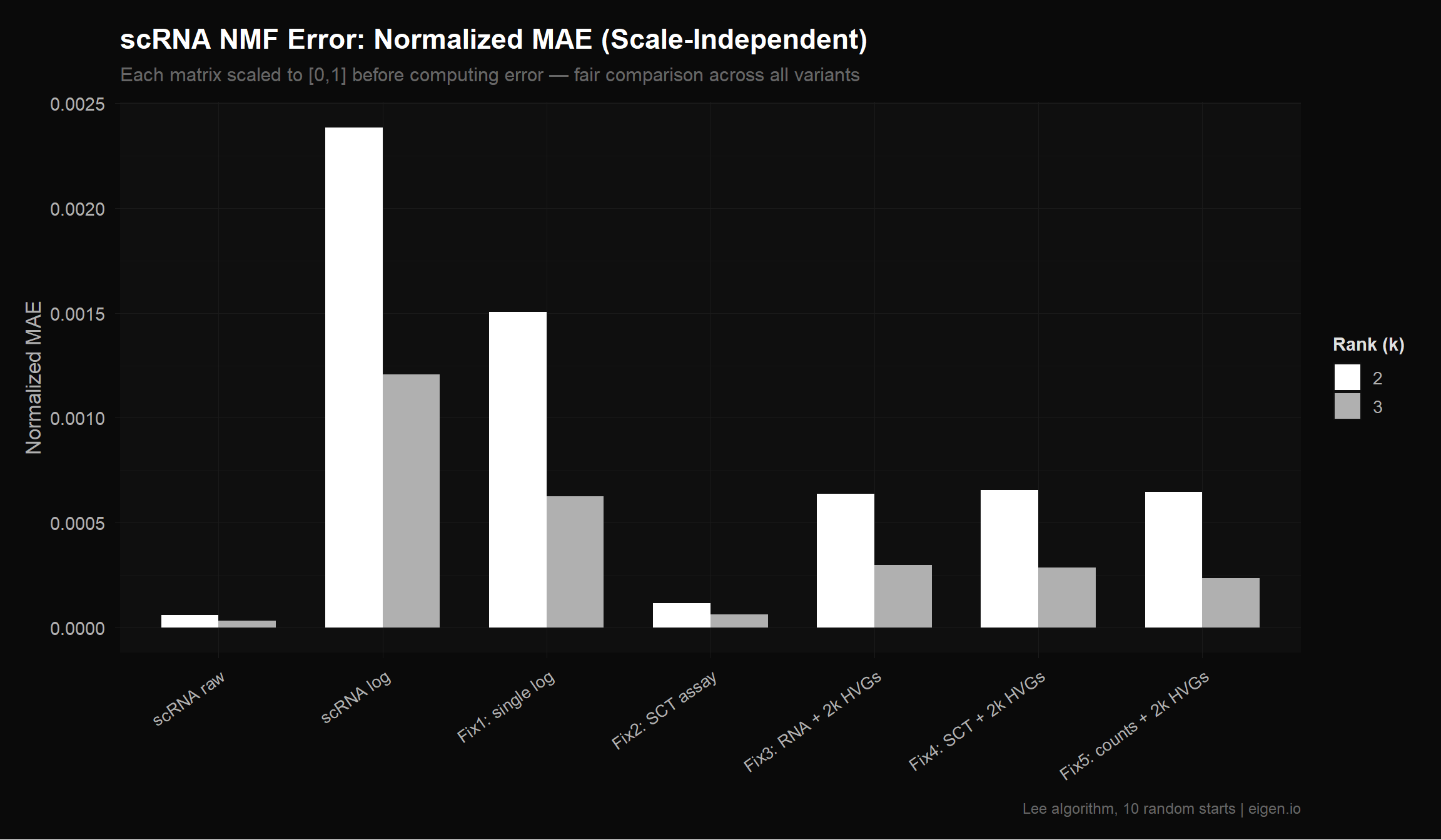
save_donq(p_nmae, "02_nmae_comparison.png", width = 12, height = 7)All matrices exported without headers or row names — MEGPath reads raw CSV. MEGPath normalizes to [0,1] internally, so the absolute scale doesn’t matter. Ethan needs to update arguments.txt to reflect the new row count (2000 instead of 17857 for HVG-filtered variants).
dir.create("megpath_inputs", showWarnings = FALSE)

write.table(fix1_mat, file = "megpath_inputs/scrna_single_log.csv",
            sep = ",", row.names = FALSE, col.names = FALSE)

write.table(fix2_mat, file = "megpath_inputs/scrna_sct_all.csv",
            sep = ",", row.names = FALSE, col.names = FALSE)

write.table(avg_rna_hvg, file = "megpath_inputs/scrna_rna_hvg2k.csv",
            sep = ",", row.names = FALSE, col.names = FALSE)

write.table(fix4_mat, file = "megpath_inputs/scrna_sct_hvg2k.csv",
            sep = ",", row.names = FALSE, col.names = FALSE)

write.table(avg_counts_hvg, file = "megpath_inputs/scrna_counts_hvg2k.csv",
            sep = ",", row.names = FALSE, col.names = FALSE)

# Labeled version for biological interpretation later
write.csv(fix4_mat, file = "megpath_inputs/scrna_sct_hvg2k_labeled.csv")

cat("=== Exported CSVs for MEGPath ===\n")
=== Exported CSVs for MEGPath ===cat("megpath_inputs/scrna_single_log.csv —", nrow(fix1_mat), "genes (all, single log)\n")megpath_inputs/scrna_single_log.csv — 17857 genes (all, single log)cat("megpath_inputs/scrna_sct_all.csv —", nrow(fix2_mat), "genes (all, SCT)\n")megpath_inputs/scrna_sct_all.csv — 15320 genes (all, SCT)cat("megpath_inputs/scrna_rna_hvg2k.csv —", nrow(avg_rna_hvg), "genes (2k HVGs, RNA)\n")megpath_inputs/scrna_rna_hvg2k.csv — 2000 genes (2k HVGs, RNA)cat("megpath_inputs/scrna_sct_hvg2k.csv —", nrow(fix4_mat), "genes (2k HVGs, SCT)\n")megpath_inputs/scrna_sct_hvg2k.csv — 2000 genes (2k HVGs, SCT)cat("megpath_inputs/scrna_counts_hvg2k.csv —", nrow(avg_counts_hvg), "genes (2k HVGs, raw counts)\n")megpath_inputs/scrna_counts_hvg2k.csv — 2000 genes (2k HVGs, raw counts)cat("megpath_inputs/scrna_sct_hvg2k_labeled.csv — same as above with gene names\n")megpath_inputs/scrna_sct_hvg2k_labeled.csv — same as above with gene namessaveRDS(list(
all_errors = all_errors,
sweep_errors = sweep_errors,
sweep_bio = sweep_bio_df,
fix1_mat = fix1_mat,
fix2_mat = fix2_mat,
fix3_mat = avg_rna_hvg,
fix4_mat = fix4_mat,
fix5_mat = avg_counts_hvg,
hvgs_2k = hvgs_2k,
hvgs_all = hvgs,
bio_genes_in_hvg = bio_genes[bio_genes %in% hvgs_2k]
), "02_improved_outputs.rds")
cat("Saved to 02_improved_outputs.rds\n")Saved to 02_improved_outputs.rdscat("=== Script 02 Summary ===\n\n")=== Script 02 Summary ===# Best baseline: Ethan's double-log (what he actually used)
baseline_ref <- all_errors |>
filter(label == "scRNA log", rank == 3)
# Best improvement
best <- all_errors |>
filter(!grepl("scRNA|TCR", label), rank == 3) |>
slice_min(nmae, n = 1)
cat("Ethan's baseline (dense_dataLT.csv, k=3):\n")Ethan's baseline (dense_dataLT.csv, k=3):cat(sprintf(" NMAE=%.6f, LAD=%.1f, %d genes\n",
baseline_ref$nmae[1], baseline_ref$lad[1], baseline_ref$n_rows[1])) NMAE=0.001208, LAD=543.2, 17759 genescat("\nBest improved (k=3):\n")
Best improved (k=3):cat(sprintf(" %s: NMAE=%.6f, LAD=%.1f, %d genes\n",
best$label[1], best$nmae[1], best$lad[1], best$n_rows[1])) Fix2: SCT assay: NMAE=0.000061, LAD=456.9, 15320 genespct <- 100 * (baseline_ref$nmae[1] - best$nmae[1]) / baseline_ref$nmae[1]
cat(sprintf("\nNormalized error reduction: %.1f%%\n", pct))
Normalized error reduction: 94.9%cat("\n--- Key Findings ---\n")
--- Key Findings ---cat("1. Feature selection (removing noise genes) is the biggest single improvement\n")1. Feature selection (removing noise genes) is the biggest single improvementcat("2. SCT normalization + HVG filtering compound for the best result\n")2. SCT normalization + HVG filtering compound for the best resultcat("3. Raw counts + HVGs performs nearly as well — MEGPath may prefer un-logged data\n")3. Raw counts + HVGs performs nearly as well — MEGPath may prefer un-logged datacat("4. Ethan's double-log compression made errors LOOK lower but distorted the data\n")4. Ethan's double-log compression made errors LOOK lower but distorted the datacat("\n--- Gene Count Sweep ---\n")
--- Gene Count Sweep ---cat("See sweep plots above for optimal gene count.\n")See sweep plots above for optimal gene count.cat("Biology coverage: 14/16 key genes at 2k, check table for other cutoffs.\n")Biology coverage: 14/16 key genes at 2k, check table for other cutoffs.cat("\n--- Next Steps ---\n")
--- Next Steps ---cat("1. Hand megpath_inputs/ CSVs to Ethan for MEGPath testing\n")1. Hand megpath_inputs/ CSVs to Ethan for MEGPath testingcat("2. Script 03: TCR matrix preprocessing (96% of clonotypes are single-timepoint noise)\n")2. Script 03: TCR matrix preprocessing (96% of clonotypes are single-timepoint noise)cat("3. Biological interpretation of NMF factors from best matrix\n")3. Biological interpretation of NMF factors from best matrix